
Not long ago, I published an article entitled “The Sound that Data Makes”. The goal was turning data — random noise in this case — into music. The hope was that by “listening” to your data, you could gain a different kind of insights, not conveyed by visualizations or tabular summaries.
This article is a deeper dive on the subject. First, I illustrate how a turn the Riemann zeta function, at the core of the Riemann conjecture, into music. It constitutes an introduction to scientific programming, the MPmath library, and complex number algebra in Python. Of course this works with any other math function. Then I explain how to use the method on real data, create both a data sound track and a data video, and combine both.
Benefits of Data Sonification
Data visualizations offer colors and shapes, allowing you to summarize multiple dimensions in one picture. Data animations (videos) go one step further, adding a time dimension. You can find many on my YouTube channel. See example here. Then, sound adds multiple dimensions: amplitude, volume and frequency over time. Producing pleasant sound, with each musical note representing a multivariate data point, is equivalent to data binning or bukectization.
Stereo and the use of multiple musical instruments (synthesized) add more dimensions. Once you have a large database of data music, you can use it for generative AI: sound generation to mimic existing datasets. Of course, musical AI art is another application, all the way to creating synthetic movies.
Implementation
Data sonification is one the projects for participants in my GenAI certification program offered here. In the remaining of this article, I describe the various steps:
- Creating the musical scale (the notes)
- Creating and transforming the data
- Plotting the sound waves
- Producing the sound track
I also included the output sound file in the last section, for you to listen and share with your colleagues.
Musical Notes
The first step, after the imports, consists of creating a musical scale: in short, the notes. You need it if you want to create a pleasant melody. Without it, the sound will feel like noise.
import numpy as np
import matplotlib as mpl
import matplotlib.pyplot as plt
from scipy.io import wavfile
import mpmath

#-- Create the list of musical notes

scale=[]
for k in range(35, 65):
    note=440*2**((k-49)/12)
    if k%12 != 0 and k%12 != 2 and k%12 != 5 and k%12 != 7 and k%12 != 10:
        scale.append(note) # add musical note (skip half tones)
n_notes = len(scale) # number of musical notes
Data production and transformation
The second step generates the data, and transforms it via rescaling, so that it can easily be turned into music. Here I use sampled values of the Dirichlet eta function (a sister of the Riemann zeta function), as input data. But you could use any real data instead. I transform the multivariate data into 3 features indexed by time: frequency (the pitch), volume also called amplitude, and the duration for each of the 300 musical notes corresponding to the data. Real and Imag are respectively the real and imaginary part of a complex number.
#-- Generate the data

n = 300
sigma = 0.5
min_t = 400000
max_t = 400020

def create_data(f, nobs, min_t, max_t, sigma):
    z_real = []
    z_imag = []
    z_modulus = []
    incr_t = (max_t - min_t) / nobs
    for t in np.arange(min_t, max_t, incr_t):
        if f == 'Zeta':
            z = mpmath.zeta(complex(sigma, t))
        elif f == 'Eta':
            z = mpmath.altzeta(complex(sigma, t))
        z_real.append(float(z.real))
        z_imag.append(float(z.imag))
        modulus = np.sqrt(z.real*z.real + z.imag*z.imag)
        z_modulus.append(float(modulus))
    return(z_real, z_imag, z_modulus)

(z_real, z_imag, z_modulus) = create_data('Eta', n, min_t, max_t, sigma)

size = len(z_real) # should be identical to nobs
x = np.arange(size)

# frequency of each note
y = z_real
min = np.min(y)
max = np.max(y)
yf = 0.999*n_notes*(y-min)/(max-min)

# duration of each note
z = z_imag
min = np.min(z)
max = np.max(z)
zf = 0.1 + 0.4*(z-min)/(max-min)

# volume of each note
v = z_modulus
min = np.min(v)
max = np.max(v)
vf = 500 + 2000*(1 - (v-min)/(max-min))
Plotting the sound waves
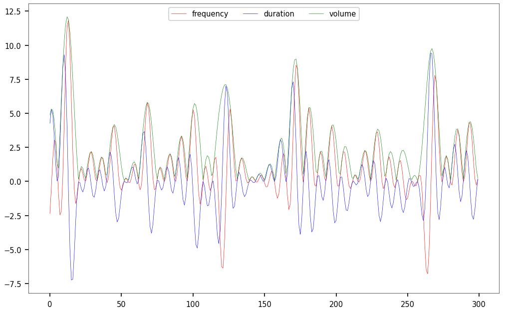
The next step plots the 3 values attached to each musical note, as 3 time series.
#-- plot data

mpl.rcParams['axes.linewidth'] = 0.3
fig, ax = plt.subplots()
ax.tick_params(axis='x', labelsize=7)
ax.tick_params(axis='y', labelsize=7)
plt.rcParams['axes.linewidth'] = 0.1
plt.plot(x, y, color='red', linewidth = 0.3)
plt.plot(x, z, color='blue', linewidth = 0.3)
plt.plot(x, v, color='green', linewidth = 0.3)
plt.legend(['frequency','duration','volume'], fontsize="7",
    loc ="upper center", ncol=3)
plt.show()
Producing the sound track
Each wave corresponds to a musical note. You turn the concatenated waves into a wav file using the wavfile.write function from the Scipy library. Other than that, there is no special sound library involved here! Hard to make it easier.
#-- Turn the data into music

def get_sine_wave(frequency, duration, sample_rate=44100, amplitude=4096):
    t = np.linspace(0, duration, int(sample_rate*duration))
    wave = amplitude*np.sin(2*np.pi*frequency*t)
    return wave

wave=[]
for t in x: # loop over dataset observations, create one note per observation
    note = int(yf[t])
    duration = zf[t]
    frequency = scale[note]
    volume = vf[t]  ## 2048
    new_wave = get_sine_wave(frequency, duration = zf[t], amplitude = vf[t])
    wave = np.concatenate((wave,new_wave))
wavfile.write('sound.wav', rate=44100, data=wave.astype(np.int16))
Results
The technical document detailing the project in question can be found here. It includes additional details on how to add an audio file such as below to a data video, as well as test datasets (from real life) to turn into sound. Perhaps the easiest way to add audio to a video is to turn the wav file into mp4 format, then use the Moviepy library to combine both. To listen to the generated music, click on the arrow in the box below.
The figure below shows the frequency, duration and volume attached to each of the 300 musical notes in the wav file, prior to re-scaling. The volume is maximum each time the Riemann zeta function hits a zero on the critical line. This is one of the connections to the Riemann Hypothesis.
About the Author

Vincent Granville is a pioneering data scientist and machine learning expert, founder of MLTechniques.com and co-founder of Data Science Central (acquired by TechTarget in 2020), former VC-funded executive, author and patent owner. Vincent’s past corporate experience includes Visa, Wells Fargo, eBay, NBC, Microsoft, CNET, InfoSpace. Vincent is also a former post-doc at Cambridge University, and the National Institute of Statistical Sciences (NISS).
Vincent published in Journal of Number Theory, Journal of the Royal Statistical Society (Series B), and IEEE Transactions on Pattern Analysis and Machine Intelligence. He is also the author of “Intuitive Machine Learning and Explainable AI”, available here. He lives in Washington state, and enjoys doing research on stochastic processes, dynamical systems, experimental math and probabilistic number theory.