
Time-series data arise in many fields including finance, signal processing, speech recognition and medicine. A standard approach to time-series problems usually requires manual engineering of features which can then be fed into a machine learning algorithm. Engineering of features generally requires some domain knowledge of the discipline where the data has originated from. For example, if one is dealing with signals (i.e. classification of EEG signals), then possible features would involve power spectra at various frequency bands, Hjorth parameters and several other specialized statistical properties.
A similar situation arises in image classification, where manually engineered features (obtained by applying a number of filters) could be used in classification algorithms. However, with the advent of deep learning, it has been shown that convolutional neural networks (CNN) can outperform this strategy. A CNN does not require any manual engineering of features. During training, the CNN learns lots of “filters” with increasing complexity as the layers get deeper, and uses them in a final classifier.
In this blog post, I will discuss the use of deep leaning methods to classify time-series data, without the need to manually engineer features. The example I will consider is the classic Human Activity Recognition (HAR) dataset from the UCI repository. The dataset contains the raw time-series data, as well as a pre-processed one with 561 engineered features. I will compare the performance of typical machine learning algorithms which use engineered features with two deep learning methods (convolutional and recurrent neural networks) and show that deep learning can surpass the performance of the former.
I have used Tensorflow for the implementation and training of the models discussed in this post. In the discussion below, code snippets are provided to explain the implementation. For the complete code, please see my Github repository.
Convolutional Neural Networks (CNN)
The first step is to cast the data in a numpy array with shape (batch_size, seq_len, n_channels) where batch_size is the number of examples in a batch during training. seq_len is the length of the sequence in time-series (128 in our case) and n_channels is the number of channels where measurements are made. There are 9 channels in this case, which include 3 different acceleration measurements for each 3 coordinate axes. There are 6 classes of activities where each observation belong to: LAYING, STANDING, SITTING, WALKING_DOWNSTAIRS, WALKING_UPSTAIRS, WALKING.
First, we construct placeholders for the inputs to our computational graph:
graph = tf.Graph()with graph.as_default(): inputs_ = tf.placeholder(tf.float32, [None, seq_len, n_channels], name = 'inputs') labels_ = tf.placeholder(tf.float32, [None, n_classes], name = 'labels') keep_prob_ = tf.placeholder(tf.float32, name = 'keep') learning_rate_ = tf.placeholder(tf.float32, name = 'learning_rate')
|
where inputs_ are input tensors to be fed into the graph whose first dimension is kept at None to allow for variable batch sizes. labels_ are the one-hot encoded labels to be predicted, keep_prob_ is the keep probability used in dropout regularization to prevent overfitting, and learning_rate_ is the learning rate used in Adam optimizer.
The convolutional layers are constructed using one-dimensional kernels that move through the sequence (unlike images where 2d convolutions are used). These kernels act as filters which are being learned during training. As in many CNN architectures, the deeper the layers get, the higher the number of filters become. Each convolution is followed by pooling layers to reduce the sequence length. Below is a simple picture of a possible CNN architecture that can be used:
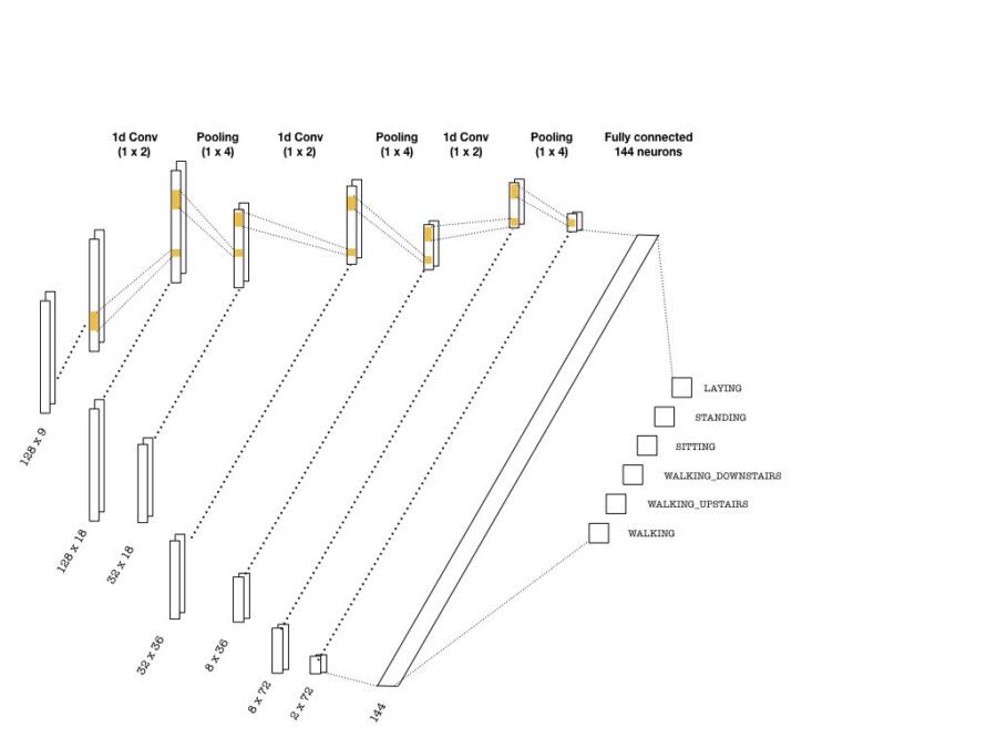
The convolutional layers depicted above are implemented as follows:
with graph.as_default(): # (batch, 128, 9) -> (batch, 32, 18) conv1 = tf.layers.conv1d(inputs=inputs_, filters=18, kernel_size=2, strides=1, padding='same', activation = tf.nn.relu) max_pool_1 = tf.layers.max_pooling1d(inputs=conv1, pool_size=4, strides=4, padding='same') # (batch, 32, 18) -> (batch, 8, 36) conv2 = tf.layers.conv1d(inputs=max_pool_1, filters=36, kernel_size=2, strides=1, padding='same', activation = tf.nn.relu) max_pool_2 = tf.layers.max_pooling1d(inputs=conv2, pool_size=4, strides=4, padding='same') # (batch, 8, 36) -> (batch, 2, 72) conv3 = tf.layers.conv1d(inputs=max_pool_2, filters=72, kernel_size=2, strides=1, padding='same', activation = tf.nn.relu) max_pool_3 = tf.layers.max_pooling1d(inputs=conv3, pool_size=4, strides=4, padding='same')
|
Once the last layer is reached, we need to flatten the tensor and feed it to a classifier with the right number of neurons (144 in the above picture). Then, the classifier outputs logits, which are used in two instances:
- Computing the softmax cross entropy, which is a standard loss measure used in multi-class problems.
- Predicting class labels from the maximum probability as well as the accuracy.
These are implemented as follows:
with graph.as_default(): # Flatten and add dropout flat = tf.reshape(max_pool_3, (-1, 2*72)) flat = tf.nn.dropout(flat, keep_prob=keep_prob_) # Predictions logits = tf.layers.dense(flat, n_classes) # Cost function and optimizer cost = tf.reduce_mean(tf.nn.softmax_cross_entropy_with_logits(logits=logits, labels=labels_)) optimizer = tf.train.AdamOptimizer(learning_rate_).minimize(cost) # Accuracy correct_pred = tf.equal(tf.argmax(logits, 1), tf.argmax(labels_, 1)) accuracy = tf.reduce_mean(tf.cast(correct_pred, tf.float32), name='accuracy')
|
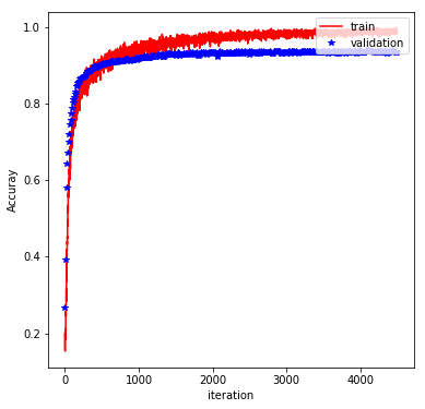
The rest of the implementation is pretty typical, and involve feeding the graph with batches of training data and evaluating the performance on a validation set. Finally, the trained model is evaluated on the test set. With the above architecture and a batch_size of 600, learning_rate of 0.001 (default value), keep_prob of 0.5, and at 500 epochs, we obtain a test accuracy of 98%. The plot below shows how the training/validation accuracy evolves through the epochs:
Long-Short-Term Memory Networks (LSTM)
LSTMs are quite popular in dealing with text based data, and has been quite successful in sentiment analysis, language translation and text generation. Since this problem also involves a sequence of similar sorts, an LSTM is a great candidate to be tried.
Below is an example architecture which can be used in our problem:
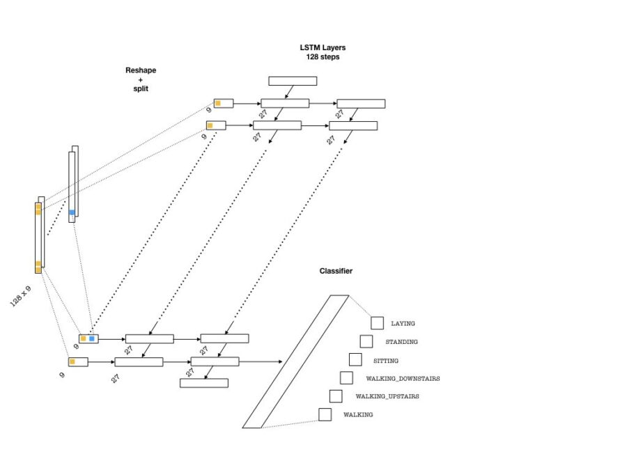
To feed the data into the network, we need to split our array into 128 pieces (one for each entry of the sequence that goes into an LSTM cell) each of shape (batch_size, n_channels). Then, a single layer of neurons will transform these inputs to be fed into the LSTM cells, each with the dimension lstm_size. This size parameter is chosen to be larger than the number of channels. This is in a way similar to embedding layers in text applications where words are embedded as vectors from a given vocabulary. Then, one needs to pick the number of LSTM layers (lstm_layers), which I have set to 2.
For the implementation, the placeholders are the same as above. The below code snippet implements the LSTM layers:
with graph.as_default(): # Construct the LSTM inputs and LSTM cells lstm_in = tf.transpose(inputs_, [1,0,2]) # reshape into (seq_len, N, channels) lstm_in = tf.reshape(lstm_in, [-1, n_channels]) # Now (seq_len*N, n_channels) # To cells lstm_in = tf.layers.dense(lstm_in, lstm_size, activation=None) # Open up the tensor into a list of seq_len pieces lstm_in = tf.split(lstm_in, seq_len, 0) # Add LSTM layers lstm = tf.contrib.rnn.BasicLSTMCell(lstm_size) drop = tf.contrib.rnn.DropoutWrapper(lstm, output_keep_prob=keep_prob_) cell = tf.contrib.rnn.MultiRNNCell([drop] * lstm_layers) initial_state = cell.zero_state(batch_size, tf.float32)There is an important technical detail in the above snippet. I reshaped the array from (batch_size, seq_len, n_channels) to (seq_len, batch_size, n_channels) first, so that tf.split would properly split the data (by the zeroth index) into a list of (batch_size, lstm_size) arrays at each step. The rest is pretty standard for LSTM implementations, involving construction of layers (including dropout for regularization) and then an initial state.
The next step is to implement the forward pass through the network and the cost function. One important technical aspect is that I included gradient clipping since it improves training by preventing exploding gradients during back propagation. Here is what the code looks like
with graph.as_default(): outputs, final_state = tf.contrib.rnn.static_rnn(cell, lstm_in, dtype=tf.float32, initial_state = initial_state) # We only need the last output tensor to pass into a classifier logits = tf.layers.dense(outputs[-1], n_classes, name='logits') # Cost function and optimizer cost = tf.reduce_mean(tf.nn.softmax_cross_entropy_with_logits(logits=logits, labels=labels_)) # Grad clipping train_op = tf.train.AdamOptimizer(learning_rate_) gradients = train_op.compute_gradients(cost) capped_gradients = [(tf.clip_by_value(grad, -1., 1.), var) for grad, var in gradients] optimizer = train_op.apply_gradients(capped_gradients) # Accuracy correct_pred = tf.equal(tf.argmax(logits, 1), tf.argmax(labels_, 1)) accuracy = tf.reduce_mean(tf.cast(correct_pred, tf.float32), name='accuracy')Notice that only the last last member of the sequence at the top of the LSTM outputs are used, since we are trying to predict one number per sequence (the class probability). The rest is similar to CNNs and we just need to feed the data into the graph to train. With lstm_size=27, lstm_layers=2, batch_size=600, learning_rate=0.0005, and keep_prob=0.5, I obtained around 95% accuracy on the test set. This is worse than the CNN result, but still quite good. It is possible that better choices of these hyperparameters would lead to improved results.
Comparison with engineered features
Previously, I have tested a few machine learning methods on this problem using the 561 pre-engineered features. One of the best performing models was a gradient booster (tree or linear), which results in an accuracy of %96 (you can read more about it from this notebook ). The CNN architecture outperforms the gradient booster, while LSTM does slightly worse.
Final Words
In this blog post, I have illustrated the use of CNNs and LSTMs for time-series classification and shown that a deep architecture can outperform a model trained on pre-engineered features. In addition to achieving better accuracy, deep learning models “engineer” their own features during training. This is highly desirable, since one does not need to have domain expertise from where the data has originated from, to be able to train an accurate model.
The sequence we used in this post was fairly small (128 steps). One may wonder what would happen if the number of steps were much larger and worry about the trainability of these architectures I discussed. One possible architecture would involve a combination of LSTM and CNN, which could work better for larger sequences (i.e. > 1000, which is problematic for LSTMs). In this case, several convolutions with pooling can effectively reduce the number of steps in the first few layers and the resulting shorter sequences can be fed into LSTM layers. An example of such an architecture has recently been used in atrial fibrillation detection from mobile device recordings.
Links
- Repository containing LSTM and CNN codes
- Please see G. Chevalier’s repo and A. Saeed’s blog where I have got lots of inspiration
- Repository containing several models trained on 561 manually generated features (in R)
- A notebook on the analysis of the data and predictions with gradient boosters (in R).
To read original blog, click here.