
The gradient decent approach is used in many algorithms to minimize loss functions. In this introduction we will see how exactly a gradient descent works. In addition, some special features will be pointed out. We will be guided by a practical example.
First of all we need a loss function. A very common approach is
 where y are the true observations of the target variable and yhat are the predictions. This function looks lika a squared function – and yes, it is. But if we assume a non linear approach for the prediction of yhat, we end up in a higher degree. In deep neural networks for example, it is a function of weights and input-features which is nonlinear.
So, lets assume that the function looks like the following polynom – as an example:
 Where f is the loss and x the weights.
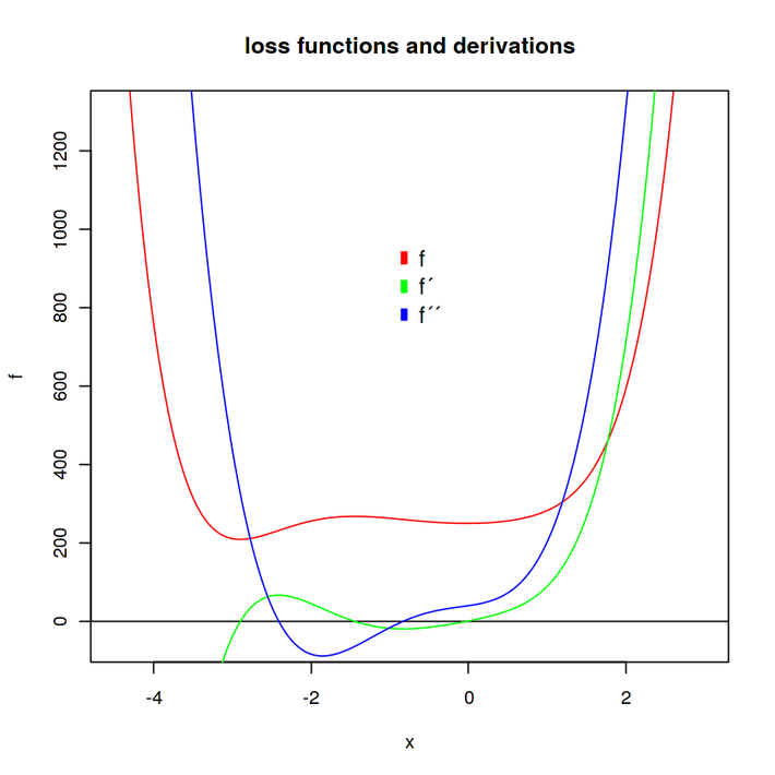
- f is the loss function
- f’ is the first derivation to x and
- f” is the second derivation to x.
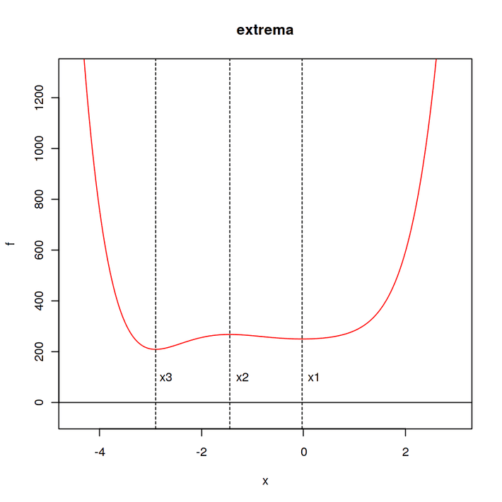
We want to find the minimum. But there are two minima and one maximum. So, firstly we find out where the extreme values are. For this intention, we use the Newton iteration approach. If we set a tangent to an arbitrary point x0 of the green function we can calculate where the linear tangent is zero instead. Through this procedure we iteratively approach the zero points of f’ and thus obtain the extrema. This intercept with x is supposed to be x1.
 When we have x1, then we start again. But now with x1.

and so forth…
To find the three points of intersection with x, we set x0 close to the suspected zero points which we can see in the function-plot.
x0 = c(1, -1, -4)
j = 1
for(x in x0) {
for (i in 1:20) {
fx = 6 * x ^ 5 + 20 * x ^ 4 + 8 * x ^ 3 + 15 * x ^ 2 + 40 * x + 1
dfx = 30 * x ^ 4 + 80 * x ^ 3 + 24 * x ^ 2 + 30 * x + 40
x = x – fx / dfx
}
assign(paste(“x”, j, sep = “”), x)
j = j + 1
}
Results are:
x1 = -0.03
x2 = -1.45
x3 = -2.9
Now that we know where f has its extrema, we can apply the gradient decent – by the way, for the gradient descent you don’t need to know where the extremes are, that’s only important for this example. To search for the minima, especially the global minimum,we apply the gradient decent.
The gradient decent is an iterative approach. It starts from initial values and moves downhill. The initial values are usually set randomly, although there are other approaches.
 Where x is for example the weight of a neuron relation and
 is the partial derivation to a certein weight. The i is the iteration index.
Why the negative learning_rate times the derivation? Well, if the derivation is positive, it means that an increase of x goes along with an increase of f and vice versa. So if the derivative is positive, x must be decreased and vice versa.
Lets start from:
x = 2
We set the learning rate to:
learning_rate = .001
for(i in 1:2000){
fx = 6*x^5+20*x^4+8*x^3+15*x^2+40*x+1
x = x – fx*learning_rate
}
Result:
Here it becomes clear why the initial values (weights) are so important. The minimum found corresponds to x1 and not x3. This is due to the initial value of x = 2. Let us now change it to:
x = -2
for(i in 1:2000){
fx = 6*x^5+20*x^4+8*x^3+15*x^2+40*x+1
x = x – fx*learning_rate
}
Result:
Well, let´s plot the first 100 x iterations:
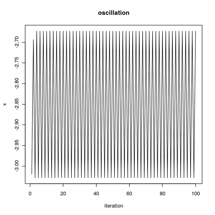 This phenomenon is called oscillation and hinders the optimization. It happens because the absolute increase f’ is same for the two opposite sides at x = -3.03 and x = -2.67:
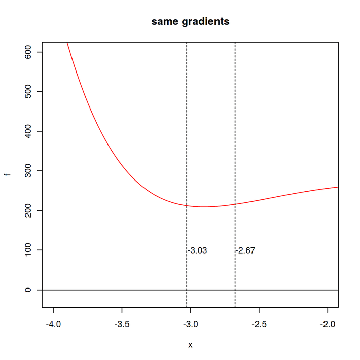 If we subtract the gradients from the opposite sides, we should get a difference of zero.
x = -2.67302
fx1 = 6*x^5+20*x^4+8*x^3+15*x^2+40*x+1
x = -3.02809
fx2 = 6*x^5+20*x^4+8*x^3+15*x^2+40*x+1
Difference is:
Learning Rate Decay
However, oscillation is not only a phenomenon that cannot be influenced, it occurs due to the chosen learning rate and the shape of the loss function. This learning rate causes the algorithm to jump from one side to the other. To counteract this, the learning rate can be reduced. Again, we start from:
x = 2
Initial learning rate:
learning_rate = .007
Learning rate decay:
decay = learning_rate / 2500; decay
0.0000028
checkX = NULL
for(i in 1:2000){
}
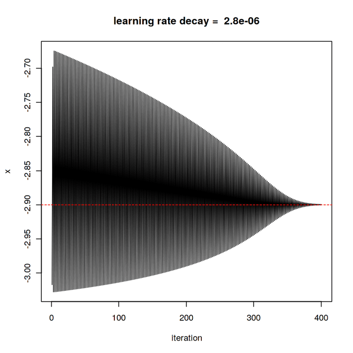
This asymmetric wedge-shaped course shows that the shrinking learning rate fulfils its task. As we know, -2.9 is the correct value.
A frequently used approach is to add a momentum term. A momentum term is the change of the value x (weight) from one iteration before:
 Where M is the weight of the momentum term. This approach is comparable to a ball rolling down the road. In the turns, it swings back with the swing it has gained. In addition, the ball rolls a bit further on flat surfaces. Lets check what happens with the oscillation when we add a momentum term.
Starting again from:
x = 2
Learning rate is again:
learning_rate = .007
M = .2
for(i in 1:2000){
x = x – fx*learning_rate + M * x_1
}
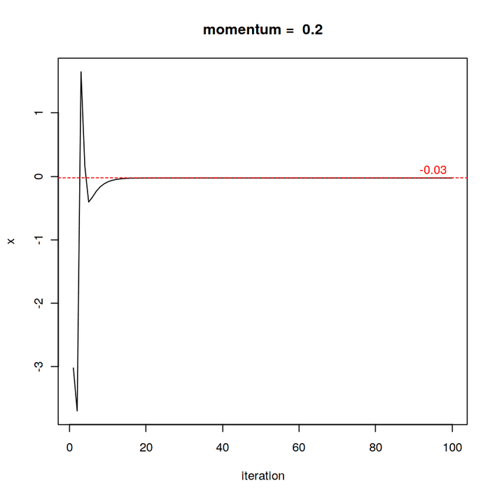
Result: