
In the last post, we talked about how to estimate the coefficients or weights of linear regression. We estimated weights which give the minimum error. Essentially it is an optimization problem where we have to find the minimum error(cost) and the corresponding coefficients. In a way, all supervised learning algorithms have optimization at the crux of it where we will have to find the model parameters which gives the minimum error(cost). In this post, I will explain some of the most commonly used methods to find the maxima or minima of the cost function.
Before starting with the cost function(average((actual -predicted)^2)), I will talk about how to find the maxima or minima of a curve. Let’s consider a curve
y= x^2 + 5x -eq(1)
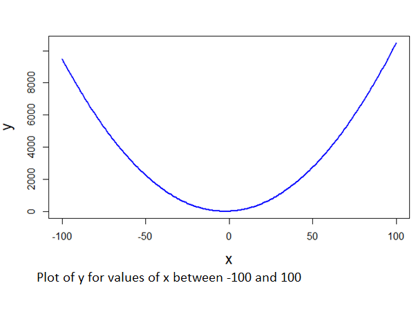
Figure 1
Let’s say we want to find the minimum point in y and value of x which gives that minimum y. There are many ways to find this. I will explain three of those.
1) Search based methods: Here the idea is to search for the minimum value of y by feeding in different values of x. There are two different ways to do this.
a) Grid search: In grid search, you give a list of values for x(as in a grid) and calculate y and see the minimum of those.
b) Random search: In this method, you randomly generate values of x and compute y and find the minimum among those.
The drawback of search based methods is that there is no guarantee that we will find a local or global minimum. Global minimum means the overall minimum of a curve. Local minimum means a point which is minimum relatively to its neighboring values.
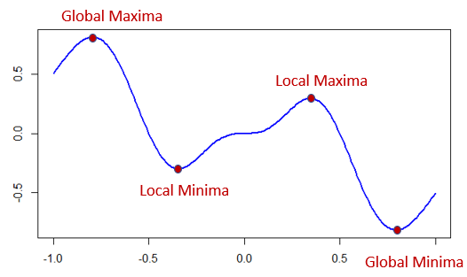
Figure 2
However, when a cost function depends on many parameters, search based methods are very useful to narrow down the search space. For example, if y was dependent on x1,x2,x3..xn, then search based methods will perform reasonably well.
2) Analytical: In analytical method, we find the point in the curve where the slope is 0. The slope of a curve is given by its derivative. Derivative of y, dy/dx, means how much y changes for a small change in x. It is same as the definition of slope. The slope is zero at the point in the curve where it is parallel to the x-axis (in the above figure all minima and maxima points have slope =0). The slope is zero for minima and maxima points. That means after finding the point where the slope is zero, we need to determine whether that point is a minima or maxima.
So in our equation 1, to find the minima of the curve, first, we need to find the point where the slope is zero. To do that we need to find the derivative of the curve and equate it to zero.
Before calculating derivative, a quick calculus refresher
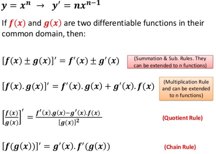
For finding the slope of our curve, we need to find the derivative of our equation(1).
y= x^2 + 5x
By summation rule,
y’ = (x^2)’ +(5x)’
==> y’ = slope of y = 2x+ 5 eq(2)
To find the point in the curve where the slope is zero, we need to equate the first derivative to zero and solve for x.
==> 2x+5=0
==> x= -5/2 = -2.5
Value of y when x = -2.5,
y= (-2.5 ^2) + 5*-2.5 = -6.25
Now we have found a point in the curve where the slope is zero. To determine whether it is a minima or maxima, we need to find the second derivative where y =0. From equation 2, y’= 2x+5. Again differentiating y’ w.r.t x,
y” = 2 eq(3)
y”(-2.5) = 2
This means the slope is positive(2) if we move slightly from the minimum point. This shows previous point(x=-2.5) was a minima point.
In general, let’s say the value of x=a after equating the first derivative to zero. To determine whether that point (known as a stationary point) is maxima or minima, find the second derivative of the function and substitute ‘a’ for x. Then,
if f ”(a)<0 then the previous point is a local maximum.
If f ”(a)>0 then the previous point is a local minimum.
Ordinary Least squared regression and its variations use the analytical method to estimate weights, which gives the minimum cost. As you might have guessed it, in order to do that we need to find the derivative of the cost function (average((actual -predicted)^2)) with respect to each of the weights and equate it to zero. For those who are interested in knowing how this can be done, I will include the details towards the end of this post.
Coming back to equation one, we have found the local minimum point. Luckily for us, this itself is the global minima, since the curve doesn’t have any other troughs. This type of curves or functions are called convex functions. It is easier to find the global minima for a convex function(using derivatives). However, for a curve as in figure 2, we might end up in a local minima. Generally, for more complex functions (eg: cost function used in neural networks), it might be unwieldy to find a minima or maxima using analytical methods.
3) Numerical: This method involves searching along the curve step by step to find the minimal point in the curve. One of the popular numerical methods is gradient descent. Many algorithms including deep learning utilize gradient descent or a variation of it. Here I will explain the working of gradient descent.
The idea of gradient descent is to move along the curve till it reaches a minima. The most common analogy is that of walking down the mountain till we reach the lowest point. There are two major aspects to consider here. Firstly how do we move along the curve i.e how do we know the next best point(starting point can be anywhere) in the curve which will direct us to the minima point. Secondly, how do we know we have reached the minima.
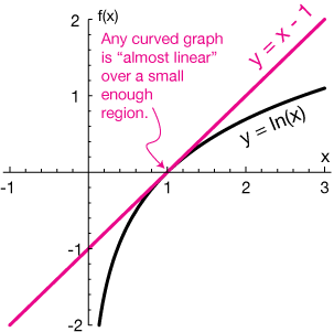
For the first aspect, we use the linear approximation. Any curve can be considered as a collection of small linear points and if we take a small linear step from a point in a curve in the direction of its slope at that point, we will still be moving along the curve. Slope at any point in a curve is given by its derivative(gradient).
The second aspect is how do we know the minima. It is easier to find the minima of a convex curve or function. Figure 1 shows a convex curve. Since there is only one minima in a convex curve, the lowest point we reach after moving along the curve will be the minima. Figure 2 is an example of a non-convex curve. Here there is no definite way of knowing whether we have reached the global minima. Generally, in these scenarios, we move along the curve for a fixed number of times and fix upon the minimum point we covered during this iteration.
Coming back to equation 1, in order to find the minimum using gradient descent we need to use the derivative which is given by equation 2. So the steps for gradient descent is as follows.
- Choose a starting value of x
- Calculate y at that point for the selected x value
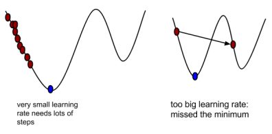
- update value of x as x= x- (alpha * y’). Here alpha is called the learning rate which controls how big a step we have to take in the direction of descent. It generally is a value less than one. If alpha is too small, it will take a long time to find the minima since we will be taking very very small steps. If alpha is too large, we may end taking big steps and miss out on the minima.

- Repeat steps 2 and 3 for a fixed number of times or till the value of y is converged i.e y remains constant for any further change in x. It means slope has become zero and x won’t be updated since y’ is zero.
R code implementation:
Defining gradient descent function which takes starting value of x, alpha and number of iterations as input
gradientDescent <- function(x, alpha, num_iters){
y_history<-as.data.frame(matrix(ncol=2,nrow=num_iters))
for (iter in 1:num_iters){
y<-x^2 +5*x;
y_history[iter,] <- c(x, y);
updates = 2*x+5;
x = x – alpha * updates;
}
y_history
}
Calling gradient descent with starting value of x as -7, alpha=0.3,number of iterations=20
res<-gradientDescent(-7,0.3,20);
cat(“Minimum point in y = “);min(res$V2)
cat(“Value of x corresponding to minimum point in y = “);res[which.min(res$V2),]$V1;
Plotting the gradient results
x<- seq(-7,2,0.01)
y<-x^2 +5*x
plot(x,y,type=”l”,col=”blue”,lwd=2,cex.lab=1.5)
points(res$V1,res$V2,type=”p”,col=”red”,lwd=2,cex.lab=1.5)
Output:
Minimum point in y = [1] -6.25
Value of x corresponding to minimum point in y = [1] -2.5
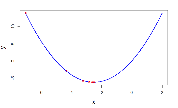
As shown in the curve when we are at a point far away from the minima, gradient values are larger. As we move closer to the minima the steps become smaller and smaller till we reach minima. Since it is a convex function there is only one minima(global minima). Therefore once minima is reached y will remain constant since gradient will be zero(i.e x will remain same). If you are interested, just change values of alpha to 1(large) and 0.001(small, increase num_iters) and see the results.
Gradinent Descent for estimating regression coefficients:
In the last post, we estimated regression coefficients using linear algebra. We estimate regression coefficients using gradient descent as well. In fact, this is the fundamental concept behind neural networks as well.
Here we will use the mtcars dataset and try to model mpg with wt and qsec variables. Equation for regression,
Y= β0X0 + β1 X1 + β2 X2 eq(4)
Y = mpg
X0 = vector of 1’s with length equal to Y
X1 = wt
X2 = qsec
Here we are trying to estimate β0,β1,β2 such that error/cost will be minimum.
Cost is defined as,
C= average(sum( ( (β0X0 + β1 X1 + β2 X2) -Y)^2) ) eq(5)
= 1/n( ∑n ( (β0X0 + β1 X1 + β2 X2-Y)^2) ), where n is the number of records and ∑n denotes sum of all records.
While we can choose any cost function, this quadratic function has nice derivatives which make it easier to find the best β’s.
An important point to note here is that cost function(function to minimize) is dependent on 3 parameters(β0,β1,β2). In the previous example for every iteration, we updated x since y was dependent on x variable alone. Here for every iteration, we have to update β0,β1,β2.
For that, we need to find the derivative of the cost function with respect to β0,β1,β2.
C'(β0) = 2/n( ∑n ((β0X0 + β1 X1 + β2 X2) – Y ) ) * X0 eq(6.1)
C'(β1) = 2/n( ∑n ((β0X0 + β1 X1 + β2 X2) – Y ) ) * X1 eq(6.2)
C'(β2) = 2/n( ∑n ((β0X0 + β1 X1 + β2 X2) – Y ) ) * X2 eq(6.3)
We get these equations by using chain rule. For one record cost function is
C = ( (β0X0 + β1 X1 + β2 X2) – Y )^2
g(x) =(β0X0 + β1 X1 + β2 X2) – Y eq(7)
f(x) = g(x)^2 eq(8)
Chain rule states that [f(g(x))]’ = f'(g(x)). g'(x). Differentiating w.r.t β0
f'(g(x))= 2. g(x) , g'(x)= X0
==> C'(β0) = 2.g(x) .X0 =2. ( (β0X0 + β1 X1 + β2 X2) – Y ) . X0
For all records,
C'(β0) = 2/n( ∑n ( (β0X0 + β1 X1 + β2 X2) – Y) ) * X0) = 2/n( ∑n ( g(x) ) * X0 )
Similarly,
C'(β1) = 2/n( ∑n ( (β0X0 + β1 X1 + β2 X2) – Y) ) * X1) = 2/n( ∑n ( g(x) ) * X0 )
C'(β2) = 2/n( ∑n ( (β0X0 + β1 X1 + β2 X2) – Y) ) * X2) = 2/n( ∑n ( g(x) ) * X0 )
Rules for finding minimum cost using gradient descent:
- Choose a starting value of β0,β1,β2
- Calculate cost at that point for the selected β0,β1,β2 values
- update rules: β0 = β0 – alpha * C'(β0) , β1 = β1 – alpha * C'(β1), β2 = β2 – alpha * C'(β2)
- repeat steps 2 and 3 for a fixed number of times or till the value of cost is converged.
R code implementation:
Before going into the code part, I want to mention just one more thing. Let’s say X is our input matrix, b the array(column vector) of all β and Y the target variable array(in this case mpg). Then β0X0 + β1 X1 + β2 X2 can be represented as X.b in matrix form where ‘.’ represents matrix multiplication.
The error e is defined as g(x) from equation 7, e = (β0X0 + β1 X1 + β2 X2) – Y . In matrix notation, this can be written as X.b -Y. The derivatives of cost w.r.t to each β can be written as (2/n)* transpose(X) .e, in which all the derivatives will be calculated in a single operation and stored as an array where the first element represents C'(β0) and the second and third element represents C'(β1) and C'(β2) respectively
Preparing dataset
attach(mtcars)
Y<- mpg
bias<-rep(1,times=length(Y))
X<-as.matrix(cbind(bias,wt,qsec))
Defining error cost and gradients function
#For calculating error, pass input matrix,beta coefficients,output y
err<-function(x,b,y){ return((x %*% b) – y )}
#For calculating cost, pass error
cost<-function(e){return((1/length(e))*crossprod(e))}
# Calculate Gradient matrix, pass input matrix and error
gradients<- function(x,e){
x<-as.matrix(x)
return((2/nrow(x))*(crossprod(x,e)))
}
Defining gradient Descent function
regression_gradient_descent=function(X,Y,converge_threshold,alpha,num_iters,print_every){
beta<-matrix(0,ncol = 1,nrow=ncol(X))
threshold<-converge_threshold
cost_vector<- c()
alpha<-alpha
error<-err(X,beta,Y)
cost_prev<-cost(error)
cost_vector<-c(cost_vector,cost_prev)
beta_prev<-beta
cost_new=cost_prev+1;cost_check<-abs(cost_new-cost_prev)
i=as.integer(0);num_iters=num_iters
print_every=ifelse(print_every >0,print_every,num_iters)
while( (cost_check > threshold) && i <=num_iters){
beta_new<- beta_prev-alpha*gradients(X,error)
error_new<-err(X,beta_new,Y)
cost_new<-cost(error_new)
cost_vector<-c(cost_vector,cost_new)
beta_prev<-beta_new
error<-error_new
cost_check<-abs(cost_new-cost_prev)
cost_prev<- cost_new
i=as.integer(i+1);
if(i%% print_every==0){print(c(i,cost_new,cost_check))}
}
list(“Beta_Estmates”=beta_new,”Cost”=cost_new,”Iterations”= i,”Cost_History”=cost_vector)
}
Here X = input matrix, Y = target variable,
converge_threshold = This is the threshold on difference between the old error and new error on each iteration. If kept zero, the function will run till it reaches a minima(local or global),
alpha = learning rate , num_iters = maximum number of iterations to run ,
print_every = It will print status for every nth value where n is the value of this argument. Status includes iteration number,cost, and cost difference with previous iteration cost
Calling gradient descent for regression
grad_reg_result<-regression_gradient_descent(X,Y,0,0.003,300000,50000)
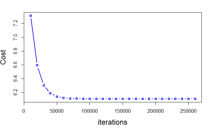
Plotting Cost iterations
j=seq(10000,grad_reg_result$Iterations,10000)
plot(j,grad_reg_result$Cost_History[j],type=”b”,col=”blue”,lwd=2,cex.lab=1.5,ylab = “Cost”,xlab=”iterations”)
Comparing beta estimates from gradient descent to lm function in R
cat(“Beta estimates using gradient Descent”);print(grad_reg_result$Beta_Estmates)
reg<-lm(mpg ~wt+qsec)
print(“Beta coffeicients from lm function”);reg$coefficients
Output:
Beta estimates using gradient Descent [,1]
bias 19.7461141
wt -5.0479774
qsec 0.9292032
[1] “Beta coffeicients from lm function”
(Intercept) wt qsec
19.746223 -5.047982 0.929198
I assume the small difference is because of the approximation differences in R. However the results are very close. One important point to remember about gradient descent is how we choose the learning rate. If it is too small, it will take forever to converge but if it is too large, we will never find a minima. From the plot above it easily understood that, in the initial stages, we were able to take big steps. As we get closer to the minima the descent starts slowing down. It is because our learning rate is static and doesn’t change throughout the entire iterations. There are different methods to overcome this problem. I will write about those in another post.
And that’s all for now. Feel free to give feedback and comments.
Have a wonderful new year guys! Cheers!