

Over the years of working on commercial AI projects, I have come across various products and business domains that have adopted machine learning algorithms. This experience helped me form some best practices for selecting the right algorithms for different types of business tasks. In this article, I will share some valuable insights from my experience regarding how to work with them in the most efficient way to meet the client’s business needs.
1. Regression
Regression is a well-known ML algorithm for exploring the relationship between independent variables or features (predictors) and a dependent variable (target) or output. Regression is usually used to explain or predict a specific numerical value based on using historical data.
How does it work in practice? Imagine that your client is a real estate business owner who wants to set the price for apartments and houses they are selling based on the best relation between price and time to sell houses. You can develop a regression model that will be able to predict the price per specified house/apartment based on various provided features in this case to have some kind of baseline recommended price.
To develop a reliable AI model, you will need to provide it with the following historical data:
- Various features that describe houses/apartments that need to be sold: the number of rooms, floors, bedrooms, and so on
- Geographical characteristics: f.e. houses in capitals are much more expensive compared with other cities
- Population, how trendy this place is, and other information that could influence price
So, let’s try to build a regression model. Given that in real life there is quite rarely a linear correlation between the target variable and all other features, let’s build polynomial regression to model a nonlinear relationship between the features and the target variable. By creating polynomial features, we can create a more complex model that can capture these nonlinear relationships.
First of all, let’s import all necessary modules and datasets that we will use for training the polynomial regression:
from sklearn.datasets import fetch_california_housing
from sklearn.linear_model import LinearRegression
from sklearn.preprocessing import PolynomialFeatures
from sklearn.model_selection import train_test_split
from sklearn.metrics import mean_squared_error

house_dataset = fetch_california_housing()
X = house_dataset.data
y = house_dataset.target
We will use the California Housing dataset, where the target variable is the median house value for California districts, expressed in hundreds of thousands of dollars ($100,000).
Then, as usual, we need to split the dataset into training and testing parts and create polynomial features. In this case, we’re using a degree of 2, which means we’ll create quadratic features.
X_train, X_test, y_train, y_test = train_test_split(X, y, test_size=0.2, random_state=12)

poly = PolynomialFeatures(degree=2)
X_train_poly = poly.fit_transform(X_train)
X_test_poly = poly.transform(X_test)
Then we need to train our model and make predictions on the test set that the model didn’t see during the training process.
model = LinearRegression()
model.fit(X_train_poly, y_train)
y_pred = model.predict(X_test_poly)
The final and obligatory step is to evaluate the model with the evaluation metric that was chosen. For our purpose, we selected MSE metrics that measure the average squared difference between the predicted and actual values. It gives higher weights to large errors, which can make it useful for detecting outliers or data points with large errors.
mse = mean_squared_error(y_test, y_pred)
print("Mean squared error:", mse)

>>> Mean squared error: 0.436677
In comparison to running a classical linear regression model without using polynomial features, the MSE error is lower (classical model has MSE = 0.53) and it has proved that you can experiment with these techniques even more for obtaining better model productivity.
2. Classification
Classification is utilized for categorizing both unstructured and structured data. Among the most common use cases of this algorithm are spam filtering, visual classification, auto-tagging, and defect detection. What other types of projects can you use it in?
Let’s say your client has a customer service department with thousands of requests per day. Helpdesk gives tags to each of the interactions with the customers. This is done for better and quicker navigation of customers’ requests and for grouping requests by topics.
To help your client to achieve their business goals, you can create a multi-label classification model that will automate the process of assigning several tags to new customer requests. The business solution will be based on previously tagged clients’ data. As a result, customer service specialists will not spend time on this activity, concentrating on more important tasks instead.
One of the problems you can face while working with the classification task in a real-life situation is unbalanced classes. An imbalance occurs when one or more classes have very low proportions in the training data as compared to the other classes. How can you combat this? There are several strategies depending on what kind of data you are working with.
- When it comes to numeric values, the problem can be solved by oversampling. Oversampling involves randomly selecting examples from the minorclass, with replacement and slight modifications, and adding them to the training dataset.
- An additional idea to overcome this issue is assigning higher weights to the minority class. So, briefly speaking, you can define the proportions of classes to improve the results.
Let’s focus on overcoming unbalancing problems in practice.
For this example, I have generated an imbalanced dataset with 64 features and 10,000 samples, where 70% of the samples belong to the majority class [0] and 30% belong to the minor class [1].
Quite a classical solution for performing classification problems could look like this:
from sklearn.model_selection import train_test_split
from sklearn.ensemble import RandomForestClassifier
from sklearn.metrics import classification_report

X, y = make_classification(n_samples=10000, n_features=64, n_informative=32, n_redundant=0, n_clusters_per_class=2, weights=[0.7, 0.3], class_sep=0.8, random_state=33)

X_train, X_test, y_train, y_test = train_test_split(X, y, test_size=0.2, random_state=33)

rf = RandomForestClassifier(n_estimators=100, random_state=33)
rf.fit(X_train, y_train)

y_pred = rf.predict(X_test)
print(classification_report(y_test, y_pred))


>>>               precision    recall  f1-score   support
>>>
>>>            0       0.85      0.99      0.91      1379
>>>            1       0.97      0.60      0.74       621

>>>     accuracy                           0.87      2000
>>>    macro avg       0.91      0.80      0.83      2000
>>> weighted avg       0.89      0.87      0.86      2000
With the resampling technique, you can oversample the minority class, undersample the majority class, or use a combination of both. This can be achieved using libraries like imbalanced-learn. Let’s look at this sample of the code with applied resampling techniques:
ros = RandomOverSampler(random_state=33)
X_resampled, y_resampled = ros.fit_resample(X_train, y_train)
We used ‘RandomOverSampler()’ from the ‘imblearn’ library to oversample the minority class in the training data. This helps balance the classes by generating synthetic data points for the minority class.
In addition to this approach, you can assign higher weights to the minority class and lower weights to the majority class. This can be done using the ‘class_weight’ parameter in the classifier. Let’s look at this part of the code:
class_weights = compute_class_weight('balanced', classes=[0, 1], y=y_resampled)Here we calculate the class weights using the ‘compute_class_weight()’ function from ‘sklearn.utils.class_weight’. Then we need to use these class weights to train our classifier.
Let’s summarize and look at the code snippet for the classification problem with resolving the problem of unbalanced classes:
from sklearn.datasets import make_classification
from sklearn.model_selection import train_test_split
from sklearn.ensemble import RandomForestClassifier
from sklearn.metrics import classification_report
from imblearn.over_sampling import RandomOverSampler
from sklearn.utils.class_weight import compute_class_weight

X, y = make_classification(n_samples=10000, n_features=64, n_informative=32, n_redundant=0, n_clusters_per_class=2, weights=[0.7, 0.3], class_sep=0.8, random_state=33)

X_train, X_test, y_train, y_test = train_test_split(X, y, test_size=0.2, random_state=33)

ros = RandomOverSampler(random_state=33)
X_resampled, y_resampled = ros.fit_resample(X_train, y_train)

class_weights = compute_class_weight('balanced', classes=[0, 1], y=y_resampled)
rf = RandomForestClassifier(n_estimators=100, random_state=33, class_weight={0: class_weights[0], 1: class_weights[1]})
rf.fit(X_resampled, y_resampled)

y_pred = rf.predict(X_test)
print(classification_report(y_test, y_pred))

>>>              precision    recall  f1-score   support

>>>            0       0.88      0.99      0.93      1379
>>>            1       0.96      0.71      0.82       621

>>>     accuracy                           0.90      2000
>>>    macro avg       0.92      0.85      0.88      2000
>>> weighted avg       0.91      0.90      0.90      2000
As you can see, comparing results obtained with and without applying techniques for preventing problems with imbalancing classes, with the second approach the metrics overall became more reliable.
3. Clustering
When it comes to clustering, this ML algorithm defines and groups unlabeled examples in datasets. Clustering uses unsupervised machine learning. This way large structured datasets can be efficiently processed and managed. At MobiDev, we commonly use clustering algorithms to bring valuable insights to businesses.
Imagine that the business owner of a supermarket chain wants to analyze employees’ performance and identify who works better and who underperforms. Numerous employees work in different supermarkets, so the owner needs to observe a full picture of employees’ performance while reducing operational costs.
To achieve this business goal, you can build a clustering model for anomaly detection. The anomaly activity is identified if employees’ behavior is uncommon (differs from all of the rest). By using the clustering model, it’s possible to identify workers whose behavior patterns are different from the rest of the employees. In this case, clustering is the first stage of the analysis to manage performance issues and productivity optimization, though a business has enough room for the implementation of other ML algorithms.
Let’s consider how anomaly detection works using clustering approaches in practice.
In the code example below, we first generate a demo dataset with 1000 samples, 3 centers, and cluster_std equals 2.5 using the ‘make_blobs()’ function from the ‘scikit-learn’ library. Then, we scale the data using the ‘StandardScaler()’ to ensure that all the features are on the same scale – it is important for the algorithms that are working based on distance.
import numpy as np
import pandas as pd
from sklearn.cluster import DBSCAN
from sklearn.datasets import make_blobs
from sklearn.preprocessing import StandardScaler
import matplotlib.pyplot as plt

# Generate a random dataset
X, y = make_blobs(n_samples=1000, centers=3, cluster_std=2.5, random_state=42)

scaler = StandardScaler()
X = scaler.fit_transform(X)
Next, we create a DBSCAN model with an ‘eps’ value of 0.3 and a ‘min_samples’ value of 5. We fit the model to the data and get the cluster labels and the number of clusters.
- ‘eps’ (short for epsilon) is the radius of the neighborhood around each data point. Points within this radius are considered neighbors of each other.
- ‘min_samples’ is the minimum number of points required to form a dense region. If a point has at least ‘min_samples’ neighbors within a distance of ‘eps’, then it is considered to be part of a dense region.
# Apply DBSCAN algorithm
dbscan = DBSCAN(eps=0.3, min_samples=5)
dbscan.fit(X)

# Obtaining model results
labels = dbscan.labels_
Then let’s plot results for validation to be sure that the algorithm worked as we expected.
# Plotting data with anomalies marked with red color

anomaly_color = '#ff0000'
plt.scatter(X[:, 0], X[:, 1], color='#006666', s=20)
plt.scatter(X[labels == -1, 0], X[labels == -1, 1], color=anomaly_color, s=40)
plt.show()
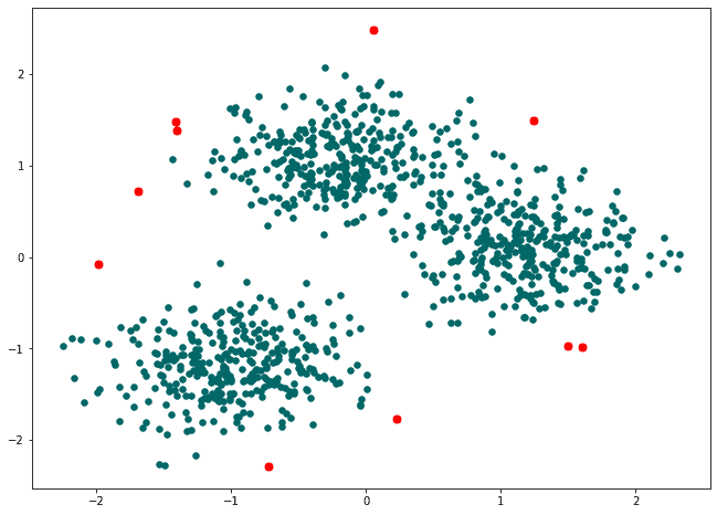
As we can see from the plot, it makes sense that anomaly detection algorithms based on clustering approach filtered out these data, so you then can remove it from dataset to clean your data before training.
Finally, we will identify the anomalies and print out the amount of anomalies that were detected.
# Identify anomalies
anomalies = X[labels == -1]
print(f"Number of anomalies: {len(anomalies)}")

>>> Number of anomalies: 10
Please note that the choice of ‘eps’ and ‘min_samples’ values will depend on the specifics of the dataset and problem at hand. You may need to experiment with different values to find the best results.
If you want to use the clustering model for identifying common patterns, anomalies can prevent your model from being effective. They can blur the whole picture, and in some cases, they need to be excluded from the model. In other words, not only identifying anomalies but also grouping the data can help to improve your model and achieve the client’s business goals.
Before Using an ML Algorithm for a Project
While the world of machine learning algorithms is exciting, it’s also full of surprises. The client doesn’t always understand what the process of turning an AI idea into a real product looks like. Here is how things can happen in the first stage of the project.
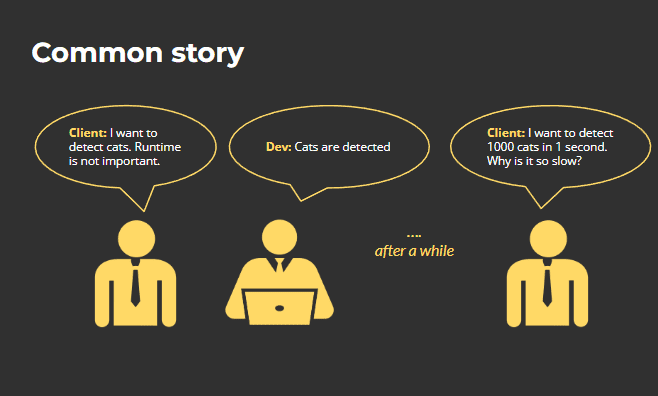
I have several tips that can help you avoid the most common pitfall of ML algorithms adoption:
- Runtime is always important, even when a client didn’t tell you about it.
- Think about speed during development. It is better to write optimized code from scratch.
- Use GPU / CPU resources at a maximum.
- Multiprocessing is a great option for parallelization.
- Write a project with the pipeline running approach — make life easier in the future when your model will be deployed.
With all the opportunities of ML algorithms, you should be really careful about how you implement them. Whichever model you choose, remember that better data is of greater significance than an algorithm, which can be enhanced by extending the training time. Good luck!
Author
Anastasiia Molodoria
AI/ML Team Leader at MobiDev.