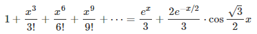
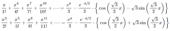
Two Beautiful Mathematical Results - Part 2

In Part 1 of this article (see here) we featured the two results below, as well as a simple way to prove these formulas.

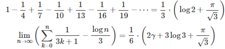
Here, we continue on the same topic, featuring and proving the formulas below, which are just the tip of the iceberg.

However cool these formulas might look, the biggest contribution here is a general framework to solve much more general problems of this type. The mathematical level is still relatively simple, accessible to people in their first year of college education, if they attended a solid course in calculus. These results are still easy to prove for people who have been exposed to the basics of complex analysis.

I haven’t seen these results published anywhere, but my guess is that they are not new. I encourage readers to post questions on Quora or Stackexchange to find more references on this topic, as Google search is of no use here.The focus here is to get more people interested in mathematics, by featuring fascinating results that are not that hard to prove, even for high school students participating in mathematical Olympiads. Also, it could be an interesting, fresh, original topic for university professors to discuss in their lectures or for exams. Finally, if you have seen many similar formulas on Wikipedia (or elsewhere), and you are wondering how they are derived, you will find the solution in this article.

The last section introduces a new, tough, unrelated problem, still unsolved today, that will be of interest to people with a background in probability and/or number theory.

1. Framework

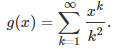
Throughout this article, I will discuss a topic that can easily be generalized, but here we only discuss the case d = 3 for simplicity. The above formulas are all a particular case of d = 3.This parameter d will become obvious very soon, and the case d = 2 is well known. The general idea is to decompose a function g(x) that has a Taylor series, into d = 3 components. It generalizes the well known decomposition into d = 2 components: The even and odd part of g. It goes as follows:

where the a‘s are the Taylor coefficients. In order to make this framework applicable to a wider class of functions (and indeed, to easily prove the above formulas), we assume that the function g has an extension to complex number arguments, and might or might not not have a Taylor series expansion. The functions g(x) = 1 / x, or g(x) = log(x), are two such examples.

Our focus in the next section is on g(x) = exp(x) where x is a complex number. We use (implicitly or explicitly) the De Moivre formula taught in high school, as far as complex number theory is concerned, and nothing beyond that level, unless otherwise stated.

2. Solution and Generalization

The first step consists of finding the d solutions of the equation z^d = 1 (z at power d) in the complex plane. This is high school level math (a simple application of De Moivre’s formula), and we will denote these complex number solutions as z_1, …, z_d, with z_1 = 1. Again, we focus here on d = 3, but the generalization to any d is straightforward. Using simple manipulations of the Taylor series for g(x) and powers of the imaginary number i, it is easy to note (say with d = 3) that g_0(x), g_1(x) and g_2(x) have the following form, illustrated here for g_1(x):

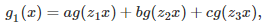
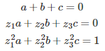
where a, b, and c are solution of the following linear system:

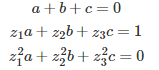
It is interesting to note that we are dealing here with a linear system associated with a Vandermonde matrix. This is important, because such a linear system has an exact, closed-form solution for any value of d. In the case d = 3, we also have: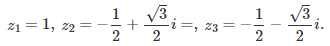

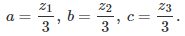
Now you have all you need to solve that linear system, and prove one of the three fascinating formulas listed in the introduction: the one corresponding to g_1(x), with g(x) = exp(x). The other two derivations proceed in a similar way. The remaining computations are cumbersome but straightforward, and can even be automated — indeed if this was one of my exam questions or competition, I would encourage participants to use automated tools to solve this system of equations. All the terms involving complex numbers eventually cancel out.

I tested my formula on a few values of x, to make sure that it was correct. It was correct up to 15 decimals, which is the maximum precision that you can get if you only use standard arithmetic. The coefficients a, b, and c, for g_1(x), are as follows: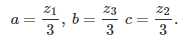

To compute the coefficients a, b, c for g_0(x), you would have to solve the following system: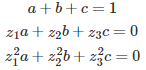

Likewise, for g_2(x), you would have to solve the following system:

In this case, the solution is

While d = 3 here, it generalizes easily to any value of d. If d = 2, the two functions g_0(x) and g_1(x) are respectively the even and odd parts of g(x), that is, g_0(x) = (g(x) + g(-x))/2 and g_1(x) = (g(x) – g(-x))/2. You can use the methodology described in this section to obtain this result. In the case d = 2, there are only two coefficients a and b, and we have z_1 = 1 and z_2 = -1, so no complex numbers are involved.

3. A More Challenging Case

Here we investigate a function g(x) that presents additional challenges — more than g(x) = exp(x) discussed earlier — though it leads to the same linear system and generic type of solution as discussed in the previous section, to compute g_0(x), g_1(x) or g_2(x). Let us consider the function g(x) defined as follows:

The key here is to realize that g satisfies the following differential equation: x g‘(x) = -log(1 – x). However, there is no simple solution in terms of elementary functions if you try to integrate it. Yet g(x) is connected with the logarithm integral function, denoted as Li(x). Finding formulas for g_0(x), g_1(x) and g_2(x) involves dealing with Li(x) in the complex plane. The solution is left as an exercise (not for beginners.)

Related article: see here. See also the Wikipedia entry on sums of reciprocals. For the sum of reciprocals of Fibonacci numbers, see here. For a generalization corresponding to any value of d, even irrational, click here.

Exercise

Apply the methodology described in the previous section, to the function g(x) = (1 + x)^p, where p is a real number (examples: p = 1/2 or p = -1.) Then redo this exercise, this time with d = 4 (easier than d = 3.)

4. Upcoming Math Problem

This problem is not related to the previous sections in this article. It offers a nice sandbox for data scientists, new research material for people interested in probability theory, and an extremely challenging problem for mathematicians and number theorists, who have worked on very similar problems for more than a hundred years, without finding a solution to this day. Here we provide a quick overview on this subject. To get an update when I will have finalized this upcoming article, sign up here to receive our newsletter.

We are interested in the following series:

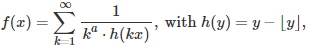
where a is a parameter greater than 1, x is a positive real number, and the brackets represent the integer part function. This series is of course divergent if x is a rational number. For which values of the parameter a and (irrational) number x is this series convergent? The problem is closely related to the convergence of the Flint Hills series, see also here. Convergence depends on how well irrational numbers can be approximated by rational numbers, and in particular, on the irrationality measure of x.

If you replace the h(kx)’s by independent random variables uniformly distributed on [0, 1], then the series represents a random variable with infinite expectation, regardless of a. Its median might exist, depending on a (if X is uniform on [0, 1] then 1 / X has a median equal to 2, but its expectation is infinite.) For an irrational number x, the sequence { kx } is equidistributed modulo 1, thus replacing h(kx) by a random variable uniformly distributed on [0, 1], seems to make sense at first glance, to study convergence. It amounts to reshuffling the terms and adding some little noise that should not impact convergence, or does it? The key here is to study the extreme value distribution (when and how close a uniform deviate approaches 0 over a large number of terms) and how well these extrema (corresponding to spikes in the chart below) are dampened by the factor k^a, as the number of terms is increasing.

For the non-random case, it seems that we have convergence if a is equal to 3 or higher. What about a = 2? No one knows. Below is a chart showing the first 2,000 terms of the series (after taking the logarithm), when a = 3 and x = SQRT(2).

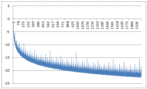
It shows that the terms in the series rapidly approach zero (the logarithm being below -20 most of the time after the first 1,500 terms), yet there are regular spikes, also decreasing in value, but these spikes are what will make the series either converge or diverge, and their behavior is governed by the parameter a, and possibly by x as well (x is assumed to be irrational here.)

Exercise

In the random case, replace the uniform distribution on [0, 1] by a uniform distribution on [-1, 1]. Now the series has positive and negative terms. How does it impact convergence?

For related articles from the same author, click here or visit www.VincentGranville.com. Follow me on on LinkedIn.

DSC Resources

Two Beautiful Mathematical Results – Part 2

Leave a Reply Cancel reply