
Natural language processing (NLP) is a broad field encompassing many different tasks such as text search, translation, named entity recognition, and topic modeling. On a daily basis, we use NLP whenever we search the internet, ask a voice assistant to tell us the weather forecast, or translate web pages written in another language. Businesses use NLP to understand how their customers talk about their product on social media. NLP may even help you receive better healthcare, as the healthcare industry applies it to electronic health records to better understand patients.
A core concern in NLP is how to best represent text data so that a computer can make use of it. In this post, I take a look at text classification to demonstrate a few common and successful methods of representing text data. While text classification has some unique characteristics — it requires labeled data, unlike other areas of NLP like topic modeling — it shares much of the text processing steps with the rest of the field. This post is aimed at analysts and data scientists familiar with modeling but new to working with text, and all of the code examples are written in Python.
If you would like to follow along with the code, you can download the dataset here . After unzipping, you’ll find a tab-delimited file called “imdb_labelled.txt” which contains a set of IMDB movie reviews and their associated sentiment (1 for positive, 0 for negative). Our task will be to predict whether a movie review was positive or negative using the text of the movie review. You can find the complete code to build a text classifier in the final section, Putting it All Together.
Organizing Your Text: Bag-of-Words
We often call text data “unstructured” because unlike data in a spreadsheet, text data isn’t naturally represented with numbers in a way that can be put into machine learning algorithms. The first step in any text classification process is transforming the text data into a structured form which we can feed into our algorithm of choice.
Bag-of-words is the simplest approach to turning text into a structured form useful for machine learning. This method translates each text document into a row that counts the number of times every word appeared in the text. This output is often called the term-document matrix. Here is what bag-of-words looks like when applied to a few (fake) movie reviews:
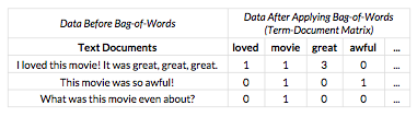
The bag-of-words procedure starts by finding the vocabulary, or all of the unique words across all of the text documents. Each unique word is assigned a column number [2]. Here, “loved” is the first column, “movie” is the second column, “great” is the third column and so on. The ellipsis indicates that there are more word columns that aren’t shown but follow the same pattern.
Once we have a column for each word in our vocabulary, we can then start counting the number of times a word appears in each text document. In the first text document, the word “great” appears 3 times, so we put a 3 in the “great” column. In the second document, “awful” appears once, so we put a 1 in the “awful” column. For words that don’t appear in a text document, we put a 0.
You might have noticed that during this transformation, we’ve lost information about word order. Once we transform “I loved this movie! It was great, great, great” into the row of data [1, 1, 3, 0, …], we can longer tell if “movie” came before or after “loved” in the original text. Whenever we use bag-of-words, we make the assumption that word order doesn’t matter. This is a bad assumption since we know a sentence like:
“She put on her shoes and left.”
has a different meaning than:
“She put on her left shoe.”
…despite the fact they use nearly the same words. Yet, in practice we can often throw away word order and still produce very useful models. If we are trying to classify whether a movie review is positive or negative, for example, word order might not matter as much as how many times someone wrote “great” or “awful” in their review.
The scikit-learn library includes a nice utility for bag-of-words called CountVectorizer. We can transform our toy IMDB dataset into a term-document matrix with just a few lines of code in Python:
import pandas as pd
 from sklearn.feature_extraction.text import CountVectorizer
filename = 'imdb_labelled.txt'
 names = ['text', 'label']
 df = pd.read_csv(filename, header=None, names=names, sep='\t', quoting=3)
bow = CountVectorizer()
 X = bow.fit_transform(df.text)
Voila! We have a term-document matrix stored in the variable X.
Finding the Words that Matter: tf-idf
A common issue we have with text analysis is that some words are much more frequent than others and aren’t useful for classification. For example, words like “the”, “is”, and “a” are common English words that don’t convey much meaning. These words will differ from task to task depending on the domain of the text documents. If we are working with movie reviews, the word “movie” will be frequent but not useful. If we were working with email data, on the other hand, the word “movie” may not be frequent and would be useful.
The simplest way to account for these overrepresented words is to divide word count by the proportion of text documents each word appeared in. For example, the document:
“I loved this movie! It was great, great, great.”
…contains the word “loved” and “movie” once each. Now, let’s suppose that we look at all the other documents and find that, in total, “loved” appears in 1% of text documents and “movie” appears in 33%. We could now weight our scores as
“loved” = times it appears in text / proportion of texts it appears in = 1 / 1%
“movie” = times it appears in text / proportion of texts it appears in = 1 / 33%
Before applying weights, both “loved” and “movie” had a score of 1 (since each word appeared in the sentence once). After we apply weights, “loved” has a score of 100 and “movie” has a score of 3. The score for “loved” is much higher relative to “movie”, indicating that we care about the word “loved” much more than “movie”.
In fact, our score for “loved” is now 33 times larger than our score for “movie”. While we suspect that “movie” should be less important than “loved” for predicting whether a review is positive or negative, this relative difference might be too big. Very rare words — perhaps, misspelled words — will receive too much relative weight in our current weighting scheme.
We need to strike a balance between downweighting very frequent words without overweighting rare words. This is what term frequency–inverse document frequency (tf-idf) weighting does for us. In the simple weighting scheme, we used the formula:
times a word appears in text * (1 / proportion of texts it appears in)
tf-idf weighting alters this formula slightly by taking the log of the second term:
times a word appears in text * log(1 / proportion of texts it appears in)
By taking the log, we ensure that our weight changes slowly in relation to how frequently a word appears in all our documents. This means that while common words are downweighted, they aren’t downweighted too much. (There’s also a connection to information theory, too).
Let’s apply tf-idf weighting to the bag-of-words matrix we built earlier. The values in the bag-of-words matrix measure the term frequency, which is the left term of the formula above. After counting the total number of documents and how many documents each word appears, we can create a matrix of weights. This is our inverse document frequency, which is the right term of the formula. Multiply these two matrices together elementwise and we create our final tf-idf weighted term-document matrix.
After applying tf-idf weighting, we’re now giving “loved”, “great” and “awful” higher importance relative to “movie”, since “movie” was so common across all text documents. These weights will help our models since they will bias the models to pay attention to what we care about and to ignore less important words.
As bag-of-words is commonly followed by tf-idf weighting, scikit-learn includes a single utility which combines both steps: TfidfVectorizer. We can replace CountVectorizer in our code above with TfidfVectorizer, and we’ll get a tf-idf weighted term-document matrix.
from sklearn.feature_extraction.text import TfidfVectorizer
tfidf = TfidfVectorizer()
 X = tfidf.fit_transform(df.text)
Working in High-Dimensional Space
As mentioned above, when using bag-of-words or tf-idf weighting, our term-document matrix has a column for each word in our vocabulary. It’s not unusual to have a vocabulary of tens of thousands of words. This means our term-document matrix will often have tens of thousands of columns or more. Such a wide matrix creates a few problems:
- Wide matrices use a large amount of computer memory.
- Having so many columns can make it difficult to train models that perform well on new, unseen data.
We can partially solve the first issue by being smart about how we store our matrix in memory. Instead of a standard matrix where we store all the values, we use a sparse matrix.In a sparse matrix, only the non-zero values are stored, and everything else is assumed to be zero. This works well for term-document matrices since each text document only uses a small subset of all the words in the vocabulary. In other words, each row in the term-document matrix will be mostly zeros, and the sparse matrix will use significantly less memory than a standard matrix.
Code that was written for standard matrices will often not handle sparse matrices without modification. Fortunately, many of scikit-learn’s algorithms support sparse matrices, making text data much easier to work with in Python. In fact, CountVectorizer and TfidfVectorizer will return sparse matrices by default, and many classifiers and regressors will handle sparse matrix inputs natively.
To address the second issue with high dimensional data (i.e. generalizability of the model), we have a few options. First of all, we can model the wide matrix directly using an algorithm like scikit-learn’s LogisticRegression. This model uses a technique called regularization to pick the columns that are relevant for classification and filter out those that aren’t. In practice, this often works well and is relatively simple to use and implement. However, it doesn’t take advantage of similarities between words.
We can potentially do better by compressing our term-document matrix before we begin to model. Instead of directly modeling a wide dataset, we first reduce the number of dimensions of our data and build a model on the much narrower dataset. This compression is very much like clustering, where a text document is assigned a score for each cluster to measure how associated it is with the cluster.
The intuition behind this idea is that we expect certain words like “enjoy,” “happy,” and “delight” to have similar meanings. Instead of including a column for each word separately, we compress them into a column that measures the broader idea of enjoyment.
This compression has the benefit of helping our models learn about related words like “enjoy,” “happy,” and “delight” simultaneously. For instance, we may have many training examples that include the word “enjoy” but only a few that include “delight.” Without compression, the model can’t learn very much about “delight” since there are so few rows to learn from. Yet, if we can squeeze “enjoy” together with “delight,” then everything our model learns about “enjoy” can also be applied to “delight.”
There are many methods to reduce the dimensionality of a term-document matrix. A very common method is to apply singular-value decomposition(SVD) to a tf-idf weighted term-document matrix. This procedure is often called latent semantic analysis (LSA). LSA is frequently used when comparing the similarity of two texts. After transforming two texts with LSA, the cosine distance between them is a good measure of their relatedness.
In text classification (and regression) we can also feed the tf-idf weighted matrix directly into a neural net to perform dimensionality reduction. In this approach, we can think of the first hidden layer as a compression step and the later layers as the classification model. The benefit to this approach — relative to LSA — is that the compression takes into account the labels we are trying to predict. In other words, the compression can ignore anything that isn’t helpful for predicting our labels.
Putting It All Together
Let’s combine the methods discussed above with a model to see what a complete text classification workflow looks like. For the model, I’ll be using a multilayer perceptron (MLP) from muffnn, a package open-sourced by Civis. This package wraps the Tensorflow neural network library in a scikit-learn interface, so we can chain our entire text classification process as a single scikit-learn Pipeline. Scikit-learn also has an MLP model, although it doesn’t include as many recent neural network techniques like dropout.
We’ll build our model using a tf-idf weighted term-document matrix as input and an indicator for whether a review was positive or negative (0 or 1) as labels. We’ll perform 5-fold cross-validation and average the out-of-sample accuracies to measure how well our model performs on new, unseen data.
from muffnn import MLPClassifier
 import numpy as np
 import pandas as pd
 from sklearn.feature_extraction.text import TfidfVectorizer
 from sklearn.model_selection import cross_val_score
 from sklearn.pipeline import make_pipeline
# Read Data. Source:
 # http://archive.ics.uci.edu/ml/machine-learning-databases/00331/sent...
filename = 'imdb_labelled.txt'
 names = ['text', 'label']
 df = pd.read_csv(filename, header=None, names=names, sep='\t', quoting=3)
# Chain together tf-idf and an MLP with a single hidden layer of size 256
 tfidf = TfidfVectorizer()
 mlp = MLPClassifier(hidden_units=(256,))
 classifier = make_pipeline(tfidf, mlp)
# Get cross-validated accuracy of the model
 cv_accuracy = cross_val_score(classifier, df.text, df.label, cv=5)
 print("Mean Accuracy: {}".format(np.mean(cv_accuracy)))
Great! This model achieves a respectable accuracy of around 78% across the 5 cross-validation folds. From here we can start to build out a more robust framework for modeling, including tuning our model parameters with grid search and following best practices such as holding out some data as a final validation of the model. After tuning our model, we can likely do better than 78% accuracy, although we probably won’t ever achieve 100% due to inconsistencies in what people consider positive and negative.
We can do a lot with text classifiers, from analyzing customer reviews to filtering spam to detecting fraud. Yet since text data doesn’t come in a ready-to-use spreadsheet format, it can often go unused. This blog post shows a few ways to shape text into a form we can plug in our favorite models. With tools like scikit-learn and Tensorflow, it’s easier than ever to get started.
By Keith Ingersoll, Senior Data Scientist @ Civis Analytics