
Source: here
In my previous article here, I discussed a simple way to solve complex optimization problems in machine learning. This was illustrated in the case of complex dynamical systems, involving non-linear equations in infinite dimensions, known as functional equations. These equations were solved using a fixed point algorithm, of which the Newton–Raphson method is a well known, widely used example.
These equations are typically solved numerically, as no theoretical solution is known in most cases. Nevertheless, in our case, a few examples have an exact, known solution. These examples with known solution are very useful, in the sense that they allow you to test your numerical algorithm and assess how fast it converges, or not. All the solutions were probability distributions, and in this article we introduce an even larger, generic class of problems (chaotic discrete dynamical systems) with known solution. The distributions presented here can thus be used as tests to benchmark optimization algorithms, but they also have their own interest for statistical modeling purposes, especially in risk management and extreme event modeling.
Each dynamical system discussed here (or in my previous article) comes with two distributions:
- A continuous one on [0, 1], known as the invariant distribution.
- A discrete one taking on strictly positive integer values, known as the digit distribution.
Besides, these distributions are very useful in number theory, though this will not be discussed here. The name Hurwitz and Riemann-Zeta is just a reminder of their strong connection to number theory problems such as continued fractions, approximation of irrational numbers by rational ones, the construction and distribution of the digits of random numbers in various numeration systems, and the famous Riemann Hypothesis that has a one million dollar prize attached to it. Some of this is discussed here and in some of my past MathOverflow questions. However, our focus here is applications in machine learning.
1. The Hurwitz-Riemann Zeta distribution
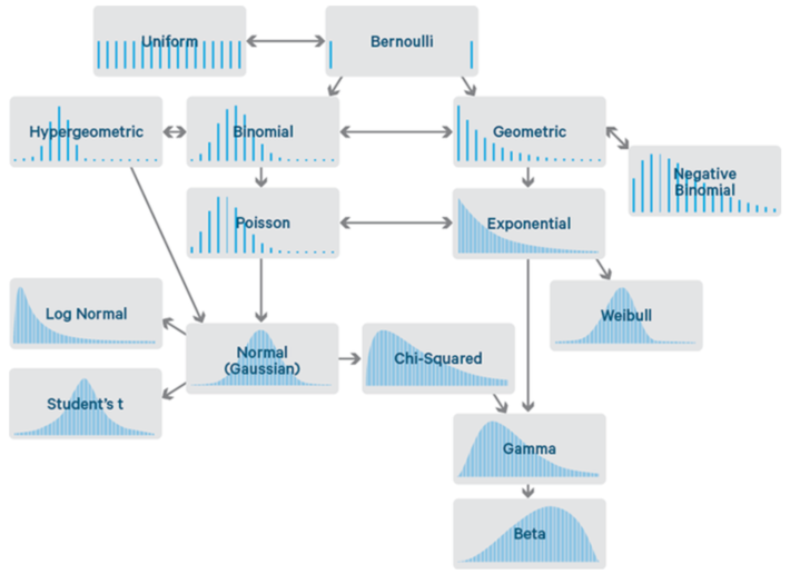
Without diving into the details, let me first briefly discuss other Riemann-related distributions invented by different authors. For a definition of the Hurwitz function, see here. It generalizes the Riemann Zeta function. The most well known probability distribution related to these functions is the discrete Zipf distribution. It is well known by machine learning practitioners, and used to model phenomena such as “the top 10 websites amount to (say) 95% of the Internet traffic”. Another example, this time continuous over the set of all positive real numbers, can be found here. The paper is entitled A New Class of Distributions Based on Hurwitz Zeta Function with Applications for Risk Management. The author defines a family of distributions that generalizes the exponential power, normal, gamma, Weibull, Rayleigh, Maxwell-Boltzmann and chi-squared distributions, with applications in actuarial sciences. Finally, there is also a well known example (for mathematicians) defined on the complex plane, see here. The paper is entitled A complete Riemann zeta distribution and the Riemann hypothesis.
Our Hurwitz-Riemann Zeta distribution is yet another example arising this time from discrete dynamical systems, continuous on [0, 1]. It also has a sister discrete distribution attached to it, useful for statistical modeling. It is defined as follows.
1.1. Our Hurwitz-Riemann Zeta distribution
The distribution discussed here is the most basic example, from the generic family described in section 2. It depends on one parameter s > 0, and the support domain is [0, 1]. The construction mechanism is defined in section 2, for the general case. Our Hurwitz-Riemann zeta distribution has the following density:
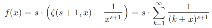
where ζ(s, x) is the Hurwitz function, see here. It has the following two first moments:
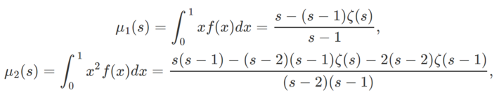
where ζ(s) = ζ(s, 1) is the Riemann Zeta function. This allows you to compute its variance. Higher moments can also be computed exactly. The cases s = 0, 1 or 2 are limiting cases, with the limit as s tends to zero, corresponding to the uniform density on [0, 1]. Particular values (s = 1, 2), empirically verified, are:
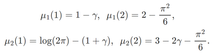
Here γ = 0.57721… is the Euler-Mascheroni constant, see here.
1.2. The discrete version
These systems also have a discrete distribution attached to them, called the digit distribution, and described in section 2. For the Hurwitz-Riemann case, the probability that a digit is equal to k, is
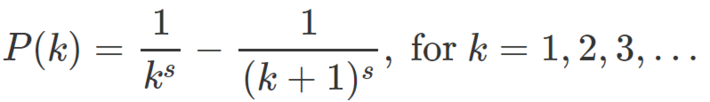
The expectation is finite only if s > 1. Likewise, the variance is finite only if s > 2. By contrast, the Zipf distribution has P(k) = (1 / ζ(s)) * 1 / k^s.
2. A generic family of distributions, with applications
We are dealing with a particular type of discrete dynamical system defined by xn+1 = p(xn) – INT(p(xn)), where INT is the integer part function, and x0 in [0, 1] is the initial condition. The function p, defined for real numbers in [0, 1], is strictly decreasing and invertible, with p(1) = 1 and p(0) infinite. The results discussed here are valid for the vast majority of initial conditions, nevertheless there are infinitely many exceptions, for instance x0 = 0. These systems are discussed in details in my previous article, here. In this section, only the main results are presented. These systems have the following properties:
- The n-th digit of x0 is dn = INT(p(xn)). These digits are called codewords in the context of dynamical systems. The probability that a digit is equal to k (k = 1, 2, 3 and so on) is F(q(k)) – F(q(k+1)) where F and q are defined below. If you know the digits, you can retrieve x0 using the algorithm described in my previous article.
- The invariant distribution F, which is the limit of the empirical distribution of the xn‘s, satisfies the following functional equation:

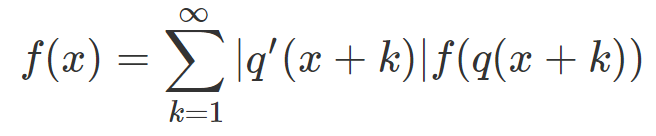
where q is the inverse of the function p, q‘ denotes the derivative of q, and f (the invariant density) is the derivative of F. We focus only on the results that are of interest to machine learning professionals.
Typically numerical methods are needed to solve the above functional equation, however here we are dealing with a large class of dynamical systems for which the theoretical solution is known. The purpose is to test numerical algorithms to check how well and how fast they can approach the exact solution, as discussed in section 2 in my previous article. The invariant distribution F discussed below is far more general than the ones described in my earlier article.
2.1. Generalized Hurwitz-Riemann Zeta distribution
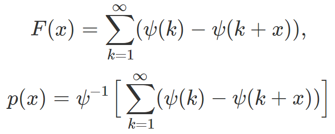
One way to find a dynamical system with know invariant distribution is to specify that distribution upfront, and then compute the resulting function p(x) that defines the system in question. Based on theory discussed here and here, one can proceed as follows. Try a monotonic increasing function r(x) with r(2) = 1 + r(1). Let F(x) = r(x+1) – r(1), and R(x) = r(x+1) – r(x). Then R(x) = F(q(x)), that is, R(p(x)) = F(x) since q(p(x)) = x. You can retrieve p(x) by inverting R(x).
A simple but generic example is
where ψ is a strictly decreasing function with ψ(∞) = 0, ψ(1) = 1, and ψ(0) = ∞. Then you have
It is easy to show that R(x) = ψ(x), thanks to a careful choice for the function r(x). This explains why the system has a simple theoretical solution; it was indeed built for that purpose. As a consequence, the probability for a digit to be equal to k (k = 1, 2, and so on) is simply equal to P(k) = ψ(k) – ψ(k+1). For more details, see Example 5 in this article, in the section Appendix 1: Exact solution for various 1-D dynamical systems.
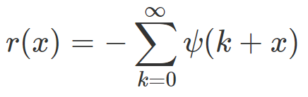
The Hurwitz-Riemann particular case in section 1.1 corresponds to
Another particular case corresponds to ψ(x) = log2(1 + 1/x), where log2 represents the logarithm in base 2. The associated dynamical system is known as the Gauss map and related to continued fractions. Its digits are the coefficients of continued fractions, and are known to follow a Gauss-Kuzmin distribution. Also, p(x) = q(x) = 1/x. It is discussed in my previous article. See also Example 2 in this article, in the section Appendix 1: Exact solution for various 1-D dynamical systems.
2.2. Application
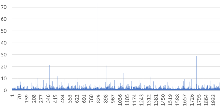
Besides being useful to test optimization algorithms against the exact solution (such as solving the above functional equation), the digits of the system have applications in simulations, encoding, random number generation, and statistical modeling. In particular, below is a picture featuring the typical behavior of the first 2,000 values of p(xn), starting with x0 = 0.5. Depending on the choice of the function ψ, these values may or may not be highly autocorrelated, and in some cases expectation and/or variance are infinite, which implies that the autocorrelation does not exist. The picture below features the Hurwitz-Riemann case with s = 2 (expectation for the digits is finite and equal to ζ(2) = π^2 / 6, but variance is infinite).
Other special distributions are discussed in my previous articles:
- New Family of Generalized Gaussian Distributions
- Interesting Application of the Poisson-Binomial Distribution
- A Strange Family of Statistical Distributions
To receive a weekly digest of our new articles, subscribe to our newsletter, here.
About the author: Vincent Granville is a data science pioneer, mathematician, book author (Wiley), patent owner, former post-doc at Cambridge University, former VC-funded executive, with 20+ years of corporate experience including CNET, NBC, Visa, Wells Fargo, Microsoft, eBay. Vincent is also self-publisher at DataShaping.com, and founded and co-founded a few start-ups, including one with a successful exit (Data Science Central acquired by Tech Target). You can access Vincent’s articles and books, here.