
Source: here
There are numerous examples in machine learning, statistics, mathematics and deep learning, requiring an algorithm to solve some complicated equations: for instance, maximum likelihood estimation (think about logistic regression or the EM algorithm) or gradient methods (think about stochastic or swarm optimization). Here we are dealing with even more difficult problems, where the solution is not a set of optimal parameters (a finite dimensional object), but a function (an infinite dimensional object).
The context is discrete, chaotic dynamical systems, with applications to weather forecasting, population growth models, complex econometric systems, image encryption, chemistry (mixtures), physics (how matter reaches an equilibrium temperature), astronomy (how celestial man-made or natural bodies end up having stable or unstable orbits), or stock market prices, to name a few. These are referred to as complex systems.
The solutions to the problems discussed here requires numerical methods, as usually no exact solution is known. The type of equation to be solved is called functional equation or stochastic integral. We explore a few cases where the exact solution is actually known: this helps assess the efficiency, accuracy and speed of convergence of the numerical methods discussed in this article. These methods are based on the fixed-point algorithm applied to infinite dimensional problems.
1. The general problem
We are dealing with a discrete dynamical system defined by xn+1 = T(xn), where T is a real-valued function, and x0 is the initial condition. For the sake of simplicity, we restrict ourselves to the case where xn is in [0, 1]. Generalizations, for instance with xn being a vector, are described here. The most well known example is the logistic map, with T(x) = λx(1-x), exhibiting a chaotic behavior or not, depending on the value of the parameter λ.
In our case, the function T(x) takes the following form: T(x) = p(x) – INT(p(x)), where INT denote the integer part function, p(x) is positive, monotonic, continuous and decreasing (thus bijective) with p(1) = 1 and p(0) infinite. For instance p(x) = 1 / x corresponds to the Gauss map associated with continued fractions; it is the most fundamental and basic example, and I discuss it here as well as below in this article. Another example is the Hurwitz-Riemann map, discussed here.
1.1. Invariant distribution and ergodicity
The invariant distribution of the system is the one followed by the successive xn‘s, or in other words, the limit of the empirical distribution attached to the xn‘s, given an initial condition x0. A lot of interesting properties can be derived if the invariant density f(x) (the derivative of the invariant distribution) is known, assuming it exists. This only works with ergodic systems. All systems under consideration here are ergodic. The invariant distribution applies to almost all initial conditions x0, though some x0‘s called exceptions, violate the law. This is a typical feature of all these systems. For some systems (the Bernoulli map for instance), the x0‘s that are not exceptions are called normal numbers.
By ergodic, I mean that for almost any initial condition x0, the sequence (xn) eventually visits all parts of [0, 1], in a uniform and random sense. This implies that the average behavior of the system can be deduced from the trajectory of a “typical” sequence (xn) attached to an initial condition x0. Equivalently, a sufficiently large collection of random instances of the process (also called orbits) can represent the average statistical properties of the entire process.
Invariant distributions are also called equilibrium or attractor distributions in probability theory.
1.2. The functional equation to be solved
Let us assume that the invariant distribution F(x) can be written as F(x) = r(x+1) − r(1) for some function r. The support domain for F(x) is [0, 1], thus F(0) = 0, F(1) = 1, F(x) = 0 if x < 0, and F(x) = 1 if x > 1. Define R(x) = r(x+1) − r(x). Then we can retrieve p(x) (under some conditions) using the formula

Thus r(x) must be increasing on [1,2] and r(2) = 1 + r(1). Not any function can be an invariant distribution.
In practice, you know p(x) and you try to find the invariant distribution F(x). So the above formula is not useful, except that it helps you create a table of dynamical systems, defined by their function p(x), with known invariant distribution. Such a table is available here, see Appendix 1 in that article, in particular example 5 featuring a Riemann zeta system. It is useful to test the fixed point algorithm described in section 2, when the exact solution is known.
If you only know p(x), to retrieve F(x) or its derivative f(x), you need to solve the following functional equation, whose unknown is the function f.
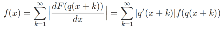
where q is the inverse of the function p. Note that R(x) = F(q(x)) or alternatively, R(p(x)) = F(x), with p(q(x)) = q(p(x)) = x. Also, here x is in [0, 1]. In practice, you get a good approximation if you use the first 1,000 terms in the sum. Typically, the invariant density f is bounded, and the weights |q‘(x+k)| are decaying relatively fast as k increases.
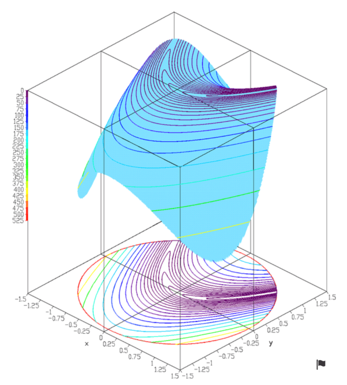
The theory behind this is beyond the scope of this article. It is based on the transfer operator, and also briefly discussed in one of my previous articles, here: see section “Functional equation for f“. The invariant density is the eigenfunction of the transfer operator, corresponding to the eigenvalue 1. Also, if x is replaced by a vector (for instance, if working with bivariate dynamical systems), the above formula can be generalized, involving two variables x, y, and the derivative of the (joint) distribution is replaced by a Jacobian.
2. Numerical solution via the fixed point algorithm
The last formula in section 1.2. suggests a simple iterative algorithm to solve this type of equation. You need to start with an initial function f0, and in this case, the uniform distribution on [0, 1] is usually a good starting point. That is, f0(x) = 1 if x is in [0, 1], and 0 elsewhere. The iterative step is as follows:
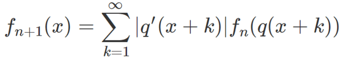
with x in [0, 1]. Each iteration n generates a whole new function fn on [0, 1], and the hope is that the algorithm converges as n tends to infinity. If convergence occurs, the limiting function must be the invariant density of the system. This is an example of the fixed point algorithm, in infinite dimension.
In practice, you compute f(x) for only (say) 10,000 values of x evenly spaced between 0 and 1. If for instance, fn+1(0.5) requires the computation of (say) fn(0.879237…) and the closest value in your array is fn(0.8792), you replace fn(0.879237…) by fn(0.8792) or you use interpolation techniques. This is more efficient than using a function defined recursively in a programming language. Surprisingly the convergence is very fast and in the examples tested, the error between the true solution and the one obtained after 3 iterations, is very small, see picture below.
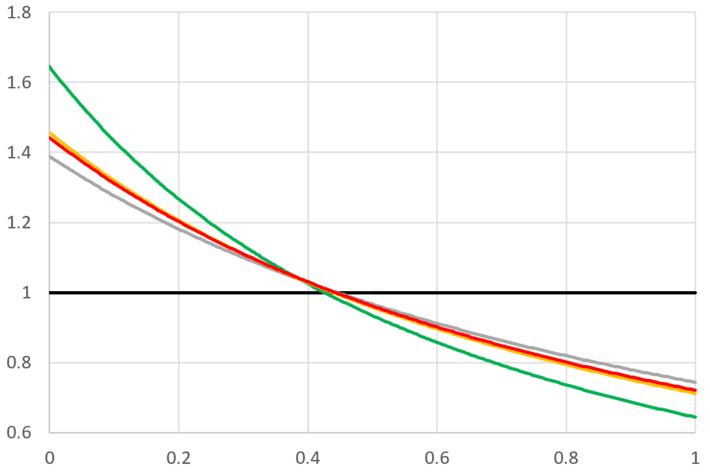 In the above picture, p(x) = q(x) = 1 / x, and the invariant distribution is known: f(x) = 1 / ((1+x)(log 2)). It is pictured in red, and it is related to the Gauss-Kuzmin distribution. Note that we started with the uniform distribution f0 pictured in black (the flat line). The first iterate f1 is in green, the second one f2 is in grey, and the third one f3 is in orange, and almost undistinguishable from the exact solution in red (I need magnifying glasses to see it). Source code for these computations is available here. In the source code, there are two extra parameters α, λ. When α = λ = 1, it corresponds to the classic case p(x) = 1 / x.
3. Applications
One interesting concept associated with these dynamical systems is that of digit. The n-th digit dn is defined as INT(p(xn)) where INT is the integer part function. I call it “digit” because all these systems have a numeration system attached to them, generalizing standard numeration systems which are just a particular case. If you know the digits attached to an initial condition x0, you can retrieve x0 with a simple algorithm. Start with n = N large enough and xn+1 = 0 (you will get about N digits of accuracy for x0), and compute iteratively xn backward from n = N to n = 0 using the recursion xn = q(xn+1 + dn) – INT(q(xn+1 + dn)). These digits can be used in encryption systems.
This will be described in detail in my upcoming book Gentle Introduction to Discrete Dynamical Systems. However, the interesting part discussed here is related to statistical modeling. As a starter, let’s look at the digits of x0 = π – 3 in two different dynamical systems:
- Continued fractions. Here p(x) = 1 / x. The first 20 digits are 7, 15, 1, 292, 1, 1, 1, 2, 1, 3, 1, 14, 3, 3, 23, 1, 1, 7, 4, 35, see here.
- A less chaotic dynamical system. Here p(x) = (-1 + SQRT(5 +4/x)) / 2. The first 20 digits are 2, 1, 1, 1, 1, 1, 1, 2, 1, 2, 1, 1, 1, 26, 1, 3, 1, 10, 1, 1. We also have F(x) = 2x / (x+1).
The distribution of the digits is known in both cases. For continued fractions, it is the Gauss-Kuzmin distribution. For the second system, the probability that a digit is equal to k, is 4 / (k(k+1)(k+2)), see Example 1 in this article. In general, the probability in question is equal to F(q(k)) – F(q(k+1)) for k = 1, 2, and so on. Clearly, the distribution of these digits can be used to quantify the level of chaos in the system. For continued fractions, the expected value of an arbitrary digit is infinite (though it is finite and well known for the logarithm of a digit, see here), while it is finite (equal to 2) for the second system. Yet each system, given enough time, will shoot arbitrarily large digits. Another way to quantify chaos in a dynamical system is to look at the auto-correlation structure of the sequence (xn). Auto-correlations very close to zero, decaying very fast, are associated with highly chaotic systems. In the case of continued fraction, the lag-1 auto-correlation, defined as the limit of the empirical auto-correlation on a sequence starting with (say) x0 = π – 3, is
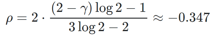
where γ is the Euler–Mascheroni constant, see Appendix 2 in this article. This is probably a new result, never published before.
Below is a picture featuring the successive values of p(xn) for the smoother dynamical system mentioned above. These values are close to the digits dn. the initial condition is x0 = π – 3. In my next article, I will further discuss a new way to define and measure chaos in these various systems.
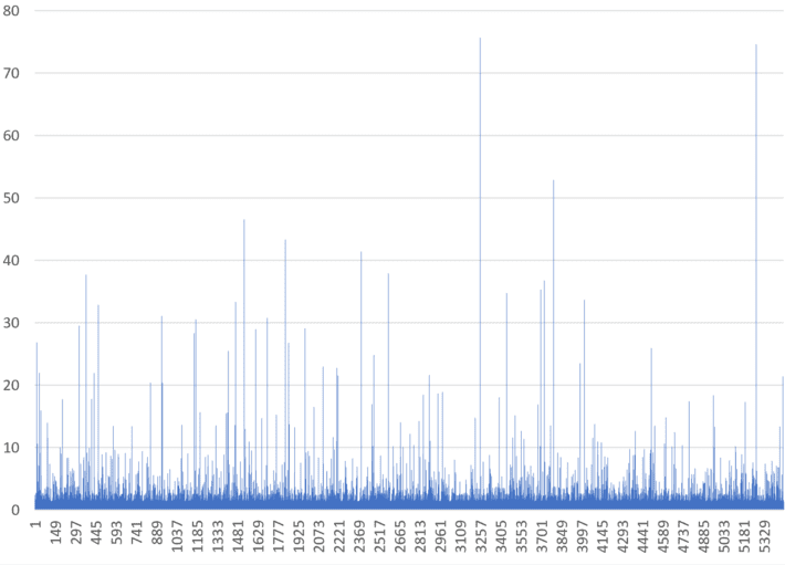
The first 5,500 values of p(xn), for n = 0, 1, 2 and so on, are featured in the above picture. Think about what business, natural or industrial process could be modeled by such kinds of time series! The possibilities are endless. For instance, it could represent meteorite hits over a large time period, with a few large values representing massive impacts. Clearly, it can be used in outlier, extreme events, and risk modeling.
Finally, here is another example, this time based on an unrelated different bivariate dynamical system on the grid (the cat map), used for image encryption. This is a mapping on a picture of a pair of cherries. The image is 74 pixels wide, and takes 114 iterations to be restored, although it appears upside-down at the halfway point (the 57th iteration). Source: here.
To receive a weekly digest of our new articles, subscribe to our newsletter, here.
About the author: Vincent Granville is a data science pioneer, mathematician, book author (Wiley), patent owner, former post-doc at Cambridge University, former VC-funded executive, with 20+ years of corporate experience including CNET, NBC, Visa, Wells Fargo, Microsoft, eBay. Vincent is also self-publisher at DataShaping.com, and founded and co-founded a few start-ups, including one with a successful exit (Data Science Central acquired by Tech Target). You can access Vincent’s articles and books, here.