
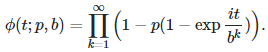
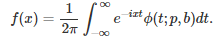
I introduce here a family of very peculiar statistical distributions governed by two parameters: p, a real number in [0, 1], and b, an integer > 1. These distributions were discovered by solving the following functional equation, corresponding to b = 2.
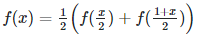
Here f(x) is the density attached to that distribution. The support domain for x is also [0, 1]. This type of distribution appears in the following context.
Let Z be an irrational number in [0, 1] (called seed) and consider the sequence x(n) = {b^n Z}. Here the brackets represent the fractional part function. In particular, INT(b x(n)) is the n-th digit of Z in base b. The values x(n) are distributed in a certain way due to the ergodicity of the underlying process. The density associated with this distribution is the function f, and for the immense majority of seeds Z, that density is uniform on [0, 1]. Seeds producing the uniform density are sometimes called normal numbers; their digit distribution is also uniform.
However, the functional equation 2f(x) = f(x/2) + f((1+x)/2) may have plenty of other solutions. Such solutions are called non-standard solutions. The set of seeds producing non-standard solutions is known to have Lebesgue measure zero, but there are infinitely many such seeds. All rational seeds are, but they produce a discrete distribution. Thus their density is of the discrete type. We are interested here in a non-discrete solution.
1. Example with p = 0.75 and b = 2
The uniform distribution corresponds to p = 0.5. By uniform, I mean uniform on the set of all normal numbers in [0, 1]. This set has its Lebesgue measure equal to 1, but it is full of holes; in particular, no rational number is a normal number.
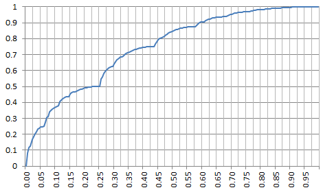
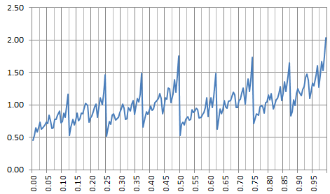
Below is a non-standard density satisfying the requirements. Actually, the plot below represents its percentile distribution. It was produced with a seed Z in [0,1] built as follows: the n-th binary digit of Z is 1 if Rand(n) < p, and 0 otherwise, using a pseudo random number generator. Here p = 0.75. Note that P.25 = 0.5 and corresponds to a dip in the chart below (P.25 denotes the 25-th percentile.) Dips are everywhere, only the big ones are visible. By contrast, the percentile distribution for the uniform (standard) case p = 0.5 is a straight line, with no dips.
2. General solution
The functional equation is a bit more complicated if b is not equal to 2. It becomes
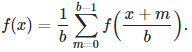
Using the construction mechanism outlined in the previous section to generate a non-standard seed Z (sometimes called a non-normal number or bad seed), it is clear that x(n) is a random variable. We also have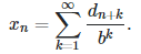 where b is the base and d(n+k) is the (n+k)-th digit of the seed Z in base b. This formula is very useful for computations. Note that Z = x(0). Furthermore, by construction, these digits are identically and independently distributed with a Bernouilli distribution of parameter p. Thus, using the convolution theorem, the characteristic function for the seed Z is
Take the derivative of the inverse Fourier transform (see section inverse formula here) and you obtain
If p = 0.5 and b = 2 we are back to the uniform case. Otherwise the solution is quite special: the density f is nowhere differentiable it seems. The support domain, though dense in [0, 1], has Lebesgue measure zero. Thus the characteristic function and density are non-standard, and would be considered improper in classical probability theory. See picture below for p = 0.55 and b = 2. See also here.
Now we should prove that this case is ergodic, for the functional equation to apply. I also tried to check with some sampled values of x to see whether 2f(x) = f(x/2) + f((1+x)/2), but the function being discontinuous everywhere, and since I got its value approximated probably to no more than two decimals, it is not easy.
3. Applications, properties and data
The distribution attached to this type of density has the following moments:
- Expectation: p / (b – 1).
- Variance: p(1 – p) / (b^2 – 1).
Why does f(x) must satisfy the functional equation discussed above? This a consequence of the fact that the underlying distribution is the equilibrium distribution for the sequence x(n) = {b x(n-1) } = {b^n Z}. In particular, the equilibrium distribution is solution to some stochastic integral equation P(X < x) = P({b X} < x). For details, see my book Applied Stochastic Processes, Chaos Modeling, and Probabilistic Properties of Numeration Systems available here, see pages 65-66.
Potential applications are found in cryptography, Fintech (stock market modeling), Bitcoin, number theory, random number generation, benchmarking statistical tests (see here) and even gaming (see here.) However, the most interesting application is probably to gain insights about how non-normal numbers look like, especially their chaotic nature. It is a fundamental tool to help solve one of the most intriguing mathematical conjectures of all times (yet unsolved): are the digits of standard constants such as Pi or SQRT(2) uniformly distributed or not? For instance, when b = 2, any departure from p = 0.5 (a normal seed) results in a strong discontinuity for f(x) at x = 0.5. If you look at the above chart, f(0) = f(1/2) = f(1) regardless of p, but discontinuities are masking this fact.
The charts featured here, as well as the underlying computations, were all produced in Excel. You can download the spreadsheet here. In particular, a very efficient algorithm is used to produce (say) one million digits of Z, and to compute one million successive values of x(n) each with a precision of 14 decimals. You can play interactively with the parameters b and p in the spreadsheet, and even try non-integer values of b (I suggest you try b = 1.5 and p = 0.5). If b < 2 is not an integer, the functional equation is more complicated: it is found in section 2.1 in this article.
Note
Another way to produce a well-behaved non-normal seed Z in base b = 2 is as follows. Let us denote as d(n, Z) the n-th binary digit of Z. Set d(n, Z) to max[ d(n, SQRT(2)/2), d(n, SQRT(3)/2) ]. Another non-normal seed is obtained as follows: d(n, Z) = max[ d(n, SQRT(2)/2), d(n + 1, SQRT(2)/2) ]. For both seeds, the theory remains applicable, and p = 3/4 (same case as the one featured in the first picture.) The reason for this is that if Z and Z‘ are two normal numbers linearly independent over the set of rational numbers, then their digits are distributed independently. Also the successive digits of Z or Z‘ behave as if they were independently distributed.
To produce 10,000 (or even millions) of digits of SQRT(2), you can use the Sagecell platform (here) with the command “N(sqrt(2),prec=10000).str(base=2)”. Or you can download the first 32 millions binary digits here (5 MB in compressed format.)