
Introduction
We propose here a simple, robust and scalable technique to perform supervised clustering on numerical data. It can also be used for density estimation, and even to define a concept of variance that is scale-invariant. This is part of our general statistical framework for data science. Previous articles included in this series are:
- Model-Free Confidence Intervals
- Tests of Hypotheses
- Hidden Decision Trees
- Jackknife Regression
- Indexation
- Fast Combinatorial Feature Selection
- The Death of the Statistical Tests of Hypotheses
General Principle: Working on the Grid, not on the Original Space
Here we discuss clustering and density estimation on the grid. The grid can be seen as an 2-dimensional or 3-dimensional array. We assume that you have selected your best predictors (for instance using our feature selection algorithm) so that the loss of yield, predictability, or accuracy, due to working in smaller dimensions, is minimum (and measurable), and is more than compensated by an increase in stability, scalability, simplicity, and robustness.
In addition, all your observations have been linearly transformed and discretized (the numerical values have been rounded) so that each observation, after this mapping, occupies a cell in the grid. For instance, if the grid associated with the data set in question consists of 1,000 columns and 2,000 rows, it can store at least 1,000 x 2,000 observations. It is OK to have two distinct but very close observations, mapped onto the same cell in the grid. Also, the worst outliers (say the top 10 most extreme points) are either ignored or put on the border of the grid, to avoid having an almost empty grid because of a few extreme ouliers. Transforming data (using log of salary rather than salary) will also help here, as in any statistical methodology. As rule of thumb #1, I suggest that 30% of the cells (in the grid) should have at least one observation attached to them. At the end of the day, you can try with different data coverage (above or below 30% of the grid) until you get optimum results based on cross-validation testing.
Note that in the above example – a 1,000 x 2,000 grid – your rounded values in your data set, once mapped onto the grid, have an accuracy above 99.9%. Most data collection processes have errors far worse than that, so the impact of discretizing your observations is almost zero, at least in most applications. Again, compare (using confusion matrices on test data from a cross-validation design) your full, exact supervised clustering system with this approximate setting, and you should not experience any significant prediction loss, in most applications.
Finally, this 1,000 x 2,000 grid (used for illustration purposes) fits easily in memory (RAM). You can even go to 4 dimensions: (say) 500 x 500 x 500 x 500 grid, and store that grid in memory, or slice it into 100 overlapping sub-grids, and do the processing with a Map-Reduce mechanism (in Hadoop for instance) on each sub-grid separately and in parallel.
For our purpose, the value of a cell in the grid will be in an integer between 0 and 255. In some cases, it could be just 0 or 1, with 1 meaning that there is a training set data point close to the location in question in the grid, 0 meaning that you are far enough away from any neighbor.
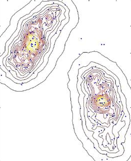
Non parametric density estimation (source: click here)
Density Estimation
We start with density estimation, as this is the base (first step) for the supervised clustering algorithm. We assume that we have g groups or classes: that is, a training set consisting of g known groups — each observation (x, y) having a label representing its group. For simplicity, let’s consider the 2-dimensional case.
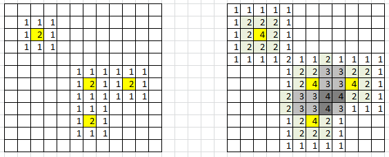
Figure 1: data points in yellow; 3×3 kernel is too small (left), 5×5 kernel is OK (right)
In figure 1, yellow cells represent locations corresponding to an actual observation (x, y) in the training set: that is, bi-variate coordinates of a point, where x could (for instance) represent the rounded monthly payment associated with a loan, and y the rounded salary, after log transformation of the salary. The groups could represent the risk level (risk of default on loan repayment), with three categories: low, medium, high.
To compute density estimates on each cell of the grid, draw a 3×3 window around each yellow cell, and add 1 to all locations (cells) in that 3×3 window. Or better, draw a 5×5 window around each yellow cell, add 1 at the center, add 2 at each location in the 3×3 sub-window, and add 1 to all locations at the border (inside) the 5×5 window. See figure 1 for illustration.
You can use bigger windows, circular windows, even infinite windows where the weight (the value added to each cell) decays exponentially fast with the distance to the center. I do not recommend it though, as it would allow you to classify any new observation (outside the training set) even if they are far away from the closest neighbor: this leads to mis-classification; such extreme observations should remain un-classified. Finally, this methodology works too in higher dimensions (3- or 4-dim).
The result is (see figure 1, right picture, for a specific group): after applying this procedure to each yellow cell and each class, you have density estimates for each class, for each cell. If we define N(z) as the value (density estimate for a specific group) computed on a particular cell z in the grid, rule of thumb #2 says that 10% of the cells with N(z) > 0 must have an N(z) that is contributed by more than one neighboring data point. In figure 1, the percentages are respectively 0% for the left picture (3×3 window), and 13/79 = 16% for the right picture (5×5 window). So clearly, the 5×5 window is OK, but the 3×3 is not. If you violate this rule, try with a bigger window, e.g. 7×7 rather than 5×5, or 5×5 rather than 3×3.
How to handle non-numeric variables?
In our example in the previous section, if one of the variables is gender (M / F) and another one is age (young / medium / old), multiply the number of groups accordingly. In our example, the number of groups (g=3: low risk, medium risk, high risk of default) will be multiplied by 2 (M / F) x 3 (young / medium / old), resulting in 18 groups, for instance “young females with medium risk of default” being one of these 18 groups.
Supervised Clustering
Now we have a straightforward classification rule: for a new data point to be classified (a point that typically does not belong to the training set), with cell location equal to z in the grid, compute the density estimate N(z | c) for each group c, then assign the point to the group c maximizing N(z | c). The speed of this algorithm is phenomenal: the computational complexity is O(g) where g is the number of groups. If you pre-classify your entire (say) 1,000 x 2,000 grid, then it is even faster, equal to O(1). You can’t beat that. Of course, accessing a cell in the grid (represented by a 2-dim array), while extremely fast and not depending on the number of observations, still requires a tiny bit of time, but it is entirely dependent only on the size of the array, and its dimension. In higher dimensions, where Map-Reduce strategies are used, more time is used to access a cell of the grid and return its value, yet it is nothing compared with the time required to perform standard supervised clustering.
Optimizing the Computations
In 2 dimensions, we have a little trick to compute the density estimates for each cell in the grid much faster, in a systematic way: it is illustrated in figure 2 below. It also works in higher dimensions, though it is most efficient in 2 dimensions.
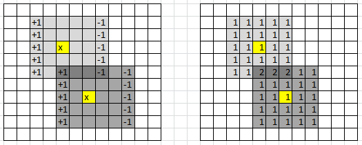
Figure 2: data points in yellow; trick to compute densities row by row, to reduce computing time
Scale-Invariant Variance
I have designed a scale-invariant variance not so long ago: you can check it out here. Interestingly, it relies on convex functions. The proof that it is always positive is based on some advanced mathematics, namely, the Jensen inequality.
Here, the purpose is a bit different. We want to create a new, scale-invariant variance, that is minimum when the data points are evenly distributed in some domain, and maximum when there are peaks and valleys or oceans of high and low density. This is still an area of intense research.
Let’s denote as N(z) the density estimate at a specific location z (cell) on the grid, as in our earlier sections. The first definition of variance that comes to mind is related to the proportion (denoted as p) of cells z with N(z) > 1, among all cells with N(z) > 0. You can now define the new variance v as v = p. It has interesting properties, but unfortunately, it is dependent on the window size (3×3 or 5×5 as in our figure 1), though this drawback can be mitigated if you abide by our two rules of thumb mentioned above. I invite you to come up with a better definition: please share your ideas in the comment section below.
Note that this new definition of variance applies to point distributions in any dimension, not just to univariate observations.
Historical Notes
This article has its origins in one of my earlier papers published in the Journal of Royal Statistical Society, series B, back in 1995: Multivariate Discriminant Analysis and Maximum Penalized Likelihood…. At that time, I was working on image analysis problems to automatically determine the proportions of various crops cultivated in several countries, based on satellite image data. This technology was cheaper than sending people in the fields to manually make the measurements via sampling – in short, it was (even back in 1995) an attempt at replacing men with robots.The same technology was used to identify tanks from enemies in the Iraq war. The images consisted of a few channels: infrared, radar, red, green, and blue — that is, about 5 dimensions. So the (x, y) coordinates mentioned earlier in this article were (in this case) color intensities in two of the 5 channels, not physical locations of a particular point.
Indeed, what we call the grid here (in this article) actually corresponds to what is referred to as the spectral space by practitioners. The actual images were referred to as the geometric or spatial space. This image remote sensing problem was very familiar to mathematicians and operations research practitioners, and was typically referred to as signal processing. And in many ways, this was a precursor to modern AI.
About the Author
Vincent Granville worked for Visa, eBay, Microsoft, Wells Fargo, NBC, a few startups and various organizations, to optimize business problems, boost ROI or to develop ROI attribution models, developing new techniques and systems to leverage modern big data and deliver added value. Vincent owns several patents, published in top scientific journals, raised VC funding, and founded a few startups. Vincent also manages his own self-funded research lab, focusing on simplifying, unifying, modernizing, automating, scaling, and dramatically optimizing statistical techniques. Vincent’s focus is on producing robust, automatable tools, API’s and algorithms that can be used and understood by the layman, and at the same time adapted to modern big, fast-flowing, unstructured data. Vincent is a post-graduate from Cambridge University.
DSC Resources
- Career: Training | Books | Cheat Sheet | Apprenticeship | Certification | Salary Surveys | Jobs
- Knowledge: Research | Competitions | Webinars | Our Book | Members Only | Search DSC
- Buzz: Business News | Announcements | Events | RSS Feeds
- Misc: Top Links | Code Snippets | External Resources | Best Blogs | Subscribe | For Bloggers
Additional Reading
- What statisticians think about data scientists
- Data Science Compared to 16 Analytic Disciplines
- 10 types of data scientists
- 91 job interview questions for data scientists
- 50 Questions to Test True Data Science Knowledge
- 24 Uses of Statistical Modeling
- 21 data science systems used by Amazon to operate its business
- Top 20 Big Data Experts to Follow (Includes Scoring Algorithm)
- 5 Data Science Leaders Share their Predictions for 2016 and Beyond
- 50 Articles about Hadoop and Related Topics
- 10 Modern Statistical Concepts Discovered by Data Scientists
- Top data science keywords on DSC
- 4 easy steps to becoming a data scientist
- 22 tips for better data science
- How to detect spurious correlations, and how to find the real ones
- 17 short tutorials all data scientists should read (and practice)
- High versus low-level data science
Follow us on Twitter: @DataScienceCtrl | @AnalyticBridge