Fractional Exponentials - Dataset to Benchmark Statistical Tests

I described here a strange type of function, that is nowhere continuous but relatively easy to integrate using probabilistic arguments. I call it the fractional part of parameter p of a function g(x), and it is denoted as g(x, p). We focus here on g(x) = exp(x). It is obtained by removing a number of terms (usually infinitely many) in the Taylor series of g(x). For instance, by removing all terms associated with an odd exponent. Examples based on g(x) = exp(x) are provided below, and explained in details in my previous article, here.

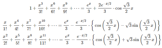
Exp(x, p) respectively for p = 8/7, p = 4/7, and p = 2/7.

More specifically, the fractional part of parameter p, where p is any real number in [0, 2], is obtained by removing the k-th term (in the Taylor series) each time the k-th digit of p in base 2, is equal to 0. The first term corresponds to k = 0. Formally, for instance if g(x) = exp(x), it is defined as follows:

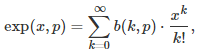
where b(k, p) is the k-th digit of p in base 2, with p in [0, 2]. This digit is equal either to 0 or 1. For instance, if p = 8/7 as in the first example (first formula in this article), then its binary digit in positions k = 0, 3, 6, 9 and so on, are all equal to 1; all other digits are 0. For any p in [0, 2], an exact formula is available for b(k, p), see here. Indeed, we have:

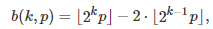
where the brackets represent the integer part function.

Curious properties of the fractional part of a function

Here we shift gears, looking at g(x, p) as a function of p, and considering x as a parameter. See Figure 1 as an illustration. This function is continuous nowhere. It is easy to notice discontinuity at p = 1, p = 3/2 or p = 3/4. Most of the time though, the jumps are too small to be noticed with the naked eye. Yet it is possible to integrate the function g(x, p) with respect to p. For instance,

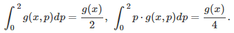
One way to easily compute these integrals, is to consider b(k, p) as independent random variables uniformly distributed on {0, 1}. Indeed, the binary digits, when averaged over p in [0, 2], exhibit the same behavior as if they were randomly distributed. This is true for all p in [0, 2] except for an infinite subset of measure 0, that includes numbers such as p = 3/4. While this seems rather intuitive, it is a consequence of the fact that almost all numbers are normal. See statement and proof of this fact here (this proof, published in 2010, is 12-page long.)

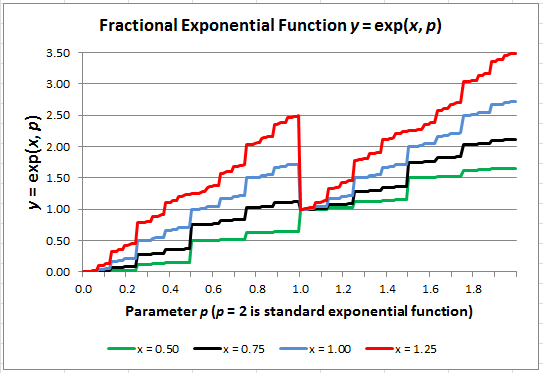
Figure 1: Fractional exponential (the X-axis represents p) computed for 4 values of x

Now if instead you integrate g(x, p) with respect to x, the result, for the indefinite integral, is G(x, p/2) where G(x) is any primitive of g(x). The result is easy to obtain by integrating the Taylor series term by term.

Benchmarking tests of statistical hypothesis

This is a great example of a “data set” that can be used to detect discontinuity points (jumps) to test how well a statistical test can identify them, and what sample sizes (number of values of exp(p, x)) are needed to detect each discontinuity. Discontinuity occurs at all values of p in [0, 2] for a given x — say x = 1/2, using g(x) = exp(x) — but for for most values of p, the jumps are very small, yet statistically significant. It also involves high precision computing to detect these smallest jumps, and also means increasing granularity, which amounts to checking a large number of p‘s to detect some of the smallest jumps. As a starting point, check out my Excel spreadsheet.

The nice feature here is that you can indefinitely increase the number of observations (p, exp(p, 1/2)) to assess the power of your tests. The data behaves like a time series, and testing amounts to detecting jumps in a time series.

Another example of infinite data set with known geometric distribution, that can be used to benchmark statistical tests (gap tests), is described here. You can even alter the data, to mimic a real enterprise data set, as follows:

Remove some data points to simulate missing data and test imputation methods
Add random noise to simulate errors, and see how it impacts your results
Add outliers to study the impact of outliers on statistical tests.

For related articles from the same author, click here or visit www.VincentGranville.com. Follow me on on LinkedIn.

DSC Resources

Fractional Exponentials – Dataset to Benchmark Statistical Tests