
This article is intended for practitioners who might not necessarily be statisticians or statistically-savvy. The mathematical level is kept as simple as possible, yet I present an original, simple approach to test for randomness, with an interesting application to illustrate the methodology. This material is not something usually discussed in textbooks or classrooms (even for statistical students), offering a fresh perspective, and out-of-the-box tools that are useful in many contexts, as an addition or alternative to traditional tests that are widely used. This article is written as a tutorial, but it also features an interesting research result in the last section.
1. Context
Let us assume that you are dealing with a time series with discrete time increments (for instance, daily observations) as opposed to a time-continuous process. The approach here is to apply and adapt techniques used for time-continuous processes, to time-discrete processes. More specifically (for those familiar with stochastic processes) we are dealing here with discrete Poisson processes. The main question that we want to answer is: Are some events occurring randomly, or is there a mechanism making the events not occurring randomly? What is the gap distribution between two successive events of the same type?
In a time-continuous setting (Poisson process) the distribution in question is modeled by the exponential distribution. In the discrete case investigated here, the discrete Poisson process turns out to be a Markov chain, and we are dealing with geometric, rather than exponential distributions. Let us illustrate this with an example.
Example
The digits of the square root of two (SQRT(2)), are believed to be distributed as if they were occurring randomly. Each of the 10 digits 0, 1, … , 9 appears with a frequency of 10% based on observations, and at any position in the decimal expansion of SQRT(2), on average the next digit does not seem to depend on the value of the previous digit (in short, its value is unpredictable.) An event in this context is defined, for example, as a digit being equal to (say) 3. The next event is the first time when we find a subsequent digit also equal to 3. The gap (or time elapsed) between two occurrences of the same digit is the main metric that we are interested in, and it is denoted as G. If the digits were distributed just like random numbers, the distribution of the gap G between two occurrences of the same digit, would be geometric, that is,
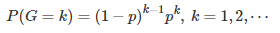
with p = 1 / 10 in this case, as each of the 10 digits (0, 1, …, 9) seems — based on observations — to have a frequency of 10%. We will show that this is indeed the case: In other words, in our example, the gap G is very well approximated by a geometric distribution of parameter p = 1 / 10, based on an analysis of the first 10 million digits of SQRT(2).
What else should I look for, and how to proceed?
Studying the distribution of gaps can reveal patterns that standard tests might fail to catch. Another statistic worth studying is the maximum gap, see this article. This is sometimes referred to as extreme events / outlier analysis. Also, in our above example, studying gaps between groups of digits (not just single digits, but for instance how frequently the “word” 234567 repeats itself in the sequence of digits, and what is the distribution of the gap for that word. For any word consisting of 6 digits, p = 1 / 1,000,000. In our case, our data set only has 10 million digits, so you may find 234567 maybe only 2 times, maybe not even once, and looking at the gap between successive occurrences of 234567, is pointless. Shorter words make more sense. This and other issues are discussed in the next section.
2. Methodology
The first step is to estimate the probabilities p associated with the model, that is, the probability for a specific event, to occur at any time. It can easily be estimated from your data set, and generally, you get a different p for each type of event. Then you need to use an algorithm to compute the empirical (observed) distribution of gaps between two successive occurrences of the same event. In our example, we have 10 types of events, each associated with the occurrence of one of the 10 digits 0, 1, …, 9 in the decimal representation of SQRT(2). The gap computation can be efficiently performed as follows:
Algorithm to compute the observed gap distribution
Do a loop over all your observations (in our case, the 10 first million digits of SQRT(2), stored in a file; each of these 10 million digits is one observation). Within the loop, at each iteration t, do:
- Let E be the event showing up in the data set, at iteration t. For instance, the occurrence of (say) digit 3 in our case. Retrieve its last occurrence stored in an array, say LastOccurrences[E]
- Compute the gap G as G = t – LastOccurrences[E]
- Update the LastOccurrences table as follows: LastOccurrences[E] = t
- Update the gap distribution table, denoted as GapTable (a two-dimensional array or better, an hash table) as follows: GapTable[E, G]++
Once you have completed the loop, all the information that you need is stored in the GapTable summary table.
Statistical testing
If some events occur randomly, the theoretical distribution of the gap, for these events, is know to be geometric, see above formula in first section. So you must test whether the empirical gap distribution (computed with the above algorithm) is statistically different from the theoretical geometric distribution of parameter p (remember that each type of event may have a different p.) If not statistically different, then the assumption of randomness should be discarded: you’ve found some patterns. This work is typically done using a Kolmogorov- Smirnov test. If you are not a statistician but instead a BI analyst or engineer, other techniques can be used instead, and are illustrated in the last section:
- You can simulate events that are perfectly randomly distributed, and compare the gap distribution obtained in your simulations, with that computed on your observations. See here how to do it, especially the last comment featuring an efficient way to do it. This Monte-Carlo simulation approach will appeal to operations research analysts.
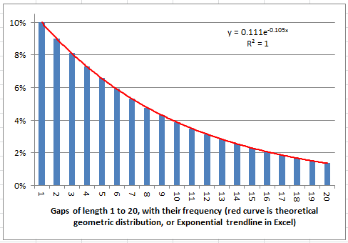
- In Excel, plot the gap distribution computed on your observations (one for each type of event), add a trendline, and optionally, display the trendline equation and its R-Squared. When choosing a trendline (model fitting) in Excel, you must select the Exponential one. This is what we did (see next section) and the good news is that, despite the very limited selection of models that Excel offers, Exponential is one of them. You can actually test other trendlines in Excel (polynomial, linear, power, or logarithmic) and you will see that by far, Exponential offers the best fit — if your events are really randomly distributed.
Further advice
If you have collected a large number of observations (say 10 million) you can do the testing on samples of increasing sizes (1,000, 10,000, 100,000 consecutive observations and so on) to see how fast the empirical distribution converges (or not) to the theoretical geometric distribution. You can also compare the behavior across samples (cross-validation), or across types of events (variance analysis). If your data set is too small (100 data points) or your events too rare (p less than 1%), consider increasing the size of your data set if possible.
Even with big data, if you are testing a large number of rare events (in our case, tons of large “words” such as occurrences 234567 rather than single digits in the decimal representation of SQRT(2)) expect many tests to result in false negatives (failure to detect true randomness.) You can even compute the probability for this to happen, assuming all your events are perfectly randomly distributed. This is known as the curse of big data.
3. Application to Number Theory Problem
Here, we further discuss the example used throughout this article to illustrate the concepts. Mathematical constants (and indeed the immense majority of all numbers) are thought to have their digits distributed as if they were randomly generated, see here for details.
Many tests have been performed on many well known constants (see here), and none of them was able to identify any departure from randomness. The gap test illustrated here is less well known, and when applied to SQRT(2), it was also unable to find departure from randomness. In fact, the fit with a random distribution, as shown in the figure below, is almost perfect.
There is a simple formula to compute any digit of SQRT(2) separately, see here, however it is not practical. Instead, we used a table of 10 million digits published here by NASA. The source claims that digits beyond the first five million have not been double-checked, so we only used the first 5 million digits. The summary gap table, methodological details, and the above picture, can be found in my spreadsheet. You can download it here.
The above chart shows a perfect fit between the observed distribution of gap lengths (averaged across the 10 digits 0, 1, …, 9) between successive occurrences of a same digit in the first 5 million decimals of SQRT(2), and the geometric distribution model, using the Exponential trendline in Excel.
I also explored the last 2 million decimals available in the NASA table, and despite the fact that they have not been double-checked, they also display the exact same random behavior. Maybe these decimals are all wrong but the mechanism that generates them preserves randomness, or maybe all or most of them are correct.
A counter-example
The number 0.123456789101112131415161718192021… known as the Champernowne constant, and obtained by concatenating the decimal representations of the natural numbers in order, has been proved to be “random”, in the sense that no digit or group of digits, occurs more frequently than any other. Such a number is known as a normal number. However, it fails miserably the gap test, with the limit distribution for the gaps (if it even exists) being totally different from a geometric distribution. I tested it on the first 8, 30, 50, 100 and 400 million decimals, and you can try too, as an exercise. All tests failed dramatically.
Ironically, no one known if SQRT(2) is a normal number, yet it passed the gap test incredibly well. Maybe a better definition of a “random” number, rather than being normal, would be a number with a geometric distribution as the limit distribution for the gaps. Can you create an artificial number that passes this test, yet exhibits strong patterns of non-randomness? Is it possible to construct a non-normal number that passes the gap test?
Potential use in cryptography
A potential application is to use digits that appear to be randomly generated (like white noise, and the digits of SQRT(2) seem to fit the bill) in documents, at random positions that only the recipient could reconstruct, perhaps three or four random digits on average for each real character in the original document, before encrypting it, to increase security — a bit like steganography. Encoding the same document a second time would result in a different kind of white noise added to the original document, and peppered randomly, each time differently — with a different intensity, and at different locations each time. This would make the task of hackers more complicated.
4. Conclusion
Finally, this is an example where intuition can be wrong, and why you need data science. In the digits of SQRT(2), while looking at the first few thousand digits (see picture below), it looked to me like it was anything but random. There were too many 99, two few 37 (among other things), according to my intuition and visual inspection (you may call it gut feelings.) It turns out that I was wrong. Look at the first few thousand digits below, chances are that your intuition will also mislead you into thinking that there are some patterns. This can be explained by the fact that patterns such as 99 are easily detected by the human brain and do stand out visually, yet in this case, they do occur with the right frequency if you use analytic tools to analyze the digits.
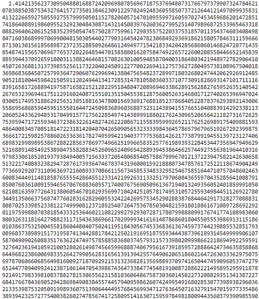
First few hundred digits or SQRT(2). Do you see any pattern?
For related articles from the same author, click here or visit www.VincentGranville.com. Follow me on on LinkedIn.
DSC Resources
- Subscribe to our Newsletter
- Comprehensive Repository of Data Science and ML Resources
- Advanced Machine Learning with Basic Excel
- Difference between ML, Data Science, AI, Deep Learning, and Statistics
- Selected Business Analytics, Data Science and ML articles
- Hire a Data Scientist | Search DSC | Classifieds | Find a Job
- Post a Blog | Forum Questions