

In part 1 here, we introduced an original class of point processes, generalizing the Poisson process which is a limiting case, in a simple and intuitive way. We started with one-dimensional processes, and then discussed the two dimensional case, when the two coordinates X and Y are paired – the equivalent of paired time series. In part 2 (this article), we continue to investigate the two-dimensional case, with unpaired coordinates: this creates a very rich class of processes, with many potential applications. We also introduce cluster processes, and statistical inference to estimate some quantities associated with these processes (granularity, radiality, variance). We also develop a general framework to identify the best model to fit with a particular data set, using non-parametric statistics, even though in many instances, we face non-identifiability issues.
We use a machine learning approach, as opposed to classic statistical methodology. It also includes the design of simple, intuitive, model-free confidence intervals. Sections 1 and 2 are found in part 1, here. Numerous simulations are provided in our interactive spreadsheet here, for replication purpose and to allow you to play with the parameters to create your own point processes, or create cluster processes to test clustering algorithms, or analyze (for instance) nearest neighbor empirical distributions. The spreadsheet will also teach you how to create scatterplots in Excel with multiple groups of data, each with a different color. This article is written for people with limited exposure to probability theory, yet goes deep into the methodology without lengthy discussions, allowing the busy practitioner or executive to grasp the concepts in a minimum amount of time. This part 2 of my article can be read independently of part 1.
3. Unpaired two-dimensional processes
Let (h, k) be any point on a 2-dimensional rectangular lattice, called the index. Typically, the lattice consists of all integer coordinates on the plane, positive or negative, and are equally spaced in both dimensions. This corresponds to a process of intensity λ = 1. A finer grid corresponds to higher intensity, while a coarser grid (for instance if h, k are even integers, positive or negative) corresponds to lower intensity, in this case λ = 1/4, as there is on average 1 point in squares with area equal to 2 x 2 = 4. Other types of grids, such as hexagonal lattices (see here) are not discussed in this article.
Let Fs be a continuous cumulative distribution function (CDF), centered at 0, symmetrical (thus the expectation is zero) with s being the core parameter. This parameter is an increasing function of the variance, with s = 0 corresponding to zero variance, and s infinite corresponding to infinite variance. To each index (h, k), we attach a point – a bivariate random vector (Xh, Yk) – with CDF Fs(x–h)Fs(y–k) = P(Xh < x, Yk < y). These points are by definition independent across the lattice, and combined together, they define our point process.
Note: The situation described here corresponds to unpaired processes. In section 2 in part 1 of this article, we worked with paired processes, with only one index k. The 2-dimensional CDF was Fs(x–k)Fs(y–k) instead. The paired processes needed to be rescaled, while the unpaired don’t, and have a more random and simpler behavior.
A logistic distribution of parameter s, or a uniform distribution on [-s, s], is typically used for Fs. The picture below shows the point process in question in plots (a) and (d), corresponding respectively to a logistic and a uniform distribution for Fs. Plots (b) and (e) are the rescaled processes; you can ignore them as they are included only for comparison purposes with paired processes investigated in part 1 (here). Plots (c) and (f) correspond respectively to a Poisson and radial process of similar intensity or variance, for comparison purposes. In theory, all these processes cover the entire plane; here only a small window appears because we are working with a finite number of index points (h, k), in the simulations. Each plot represents one realization of a point process.
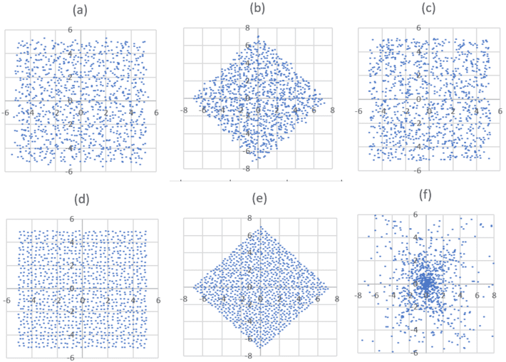
Figure 3: Unpaired process, small s
You can download the 8 MB spreadsheet from Google Doc, here. When accessing the spreadsheet on Google Doc, click on “File” at the top left corner below the spreadsheet title, then “Download”, then “Microsoft Excel” (the adapted version displayed by Google has poor graphic qualities, unlike the original version that you can get via the download in question). The spreadsheet has several tabs. The first two correspond to the paired processes described in part 1. The above Figure 3 comes from the tab “Unpaired (X, Y), small s“. The processes based on Fs, in plots (a) and (d), are called Poisson-binomial process (see part 1). When s is large, they resemble more and more to a Poisson process illustrated in plot (c), and modeling pure randomness. The striking feature here is that plot (a) and (c) represents two very different processes despite the appearances. Indeed (a) is far more related to (d) than to (c), and an appropriate test would easily determine this. Both (a) and (c) show unusual repulsion among the points: they are more evenly spaced than what true randomness would yield, which is obvious in (d) but not in (a). This is further discussed in section 5.
You can fine-tune the parameter s in the spreadsheet to obtain various configurations. See cells BC2 to BC5.
4. Cluster and hierarchical point processes
There is a simple way to combine point processes to produce clusters, and the resulting process is sometimes called an hierarchical or compound process, with the base process called the parent process, and the second level process called the child process. First, for the base process, start with (say) a Poisson-binomial process with Fs being the logistic distribution of parameter s centered at the origin (see here). Then, build the child process: in this case, a radial process such as the one in plot (f) in figure 3, around (and centered at) each point (Xh, Yk) of the base process. Another example is provided in the spreadsheet, in the “Cluster Process” tab. Figure 4 below features this example. A zoom-in is also available in the same spreadsheet, same tab.
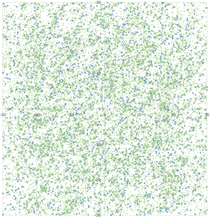
Figure 4: Cluster process
It is easy to imagine what applications such a process, with filaments, large and small conglomerates of clusters, and empty spaces, could have. Note that the blue crosses represent the parent process, that is, the points (Xh, Yk). The green points represent the child process. When s = 0, Xh = h and Yk = k. Also, I generated far more points than shown in figure 4, in a much larger window, but I only displayed a small sub-window: this is to show you how an infinite process over the entire plane would look like, once border effects (present in figure 3 but not in figure 4) no longer exist.
4.1. Radial process
The radial process attached to each blue cross in figure 4 consists of a small, random number of green points (Xi, Yi) generated as follows:
- Xi = h + ρ cos(2πΘi) log[Ui / (1 – Ui)]
- Yi = k + ρ sin(2πΘi) log[Ui / (1 – Ui)]
where Ui and Θi are uniform on [0, 1], ρ = 1, and all Θi, Ui are independent. The (Perl) source code for the generation of figure 4 is in the same spreadsheet, same tab, in column Q.
More on radial processes can be found here.
4.2. Basic cluster process
This subsection can be skipped. The purpose here is to give the beginner a simple tool to start simulating simple cluster structures, to test and benchmark cluster detection algorithms. The number of clusters can be detected using the elbow rule described in this article. There is a special tab “Cluster Basic” in my spreadsheet, to create such clusters. In addition, it shows how to produce scatterplots such as Figure 5 below, in Excel, with multiple groups, each with a different color. Other Excel features used here are conditional formatting, the NA() and the VLOOKUP() functions.
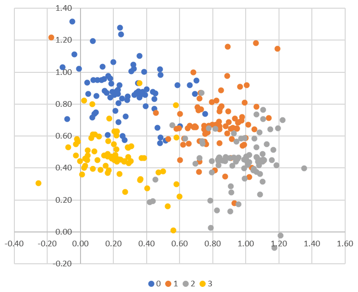
Figure 5: Simple cluster simulation
Figure 4 is also an Excel scatterplot (in the same spreadsheet, in the “Cluster process” tab) with two groups: blue and green. In the “Unpaired (X, Y), small s” tab corresponding to figure 3, another Excel feature, the used of the indirect cell referencing operator @, is used in column AX. Thus the spreadsheet can definitely teach a few tricks to the beginner.
4.3. The spreadsheet
The 8 MB spreadsheet called PoissonBinomialProcess-DSS.xlsx, is discussed in some details in the last two paragraphs of section 3, and in section 4.2. It is available here on Google Doc, for download; the preview offered by Google is of poor quality, so it is better to download the original when accessing it, by clicking on “File” (top left corner) then “Download” then “Excel Spreadsheet” on the drop-down menu.
5. Machine learning inference
So far, except in the spreadsheet, we have been dealing with Poisson-binomial processes (plots (a) and (b) in figures 1, 2, and 3) of intensity λ = 1. In any data set representing a realization of such a process, λ must be estimated and could be arbitrary. If you replace h and k by th = h/λ and tk = k/λ, now you have a Poisson-binomial process of intensity λ. The intensity represents the granularity of the process, that is, the density of points in any area.
Also here, we assume that the process covers the entire space, and that we observe points in a small window, as in Figure 4. In figure 1, 2, 3 by contrast, when simulating a realization, we used only a finite number of indices h or k, thus creating strong border effects when using a window covering almost all the points. One way to avoid most border effects in (say) figure 3, is to restrict the estimation techniques to a smaller window – a fourth of the area of the window in plots (a) or (d).
Remark: In all the cases of interest, we have Fs(x) = F1(x/s), and F1 is denoted as F. The reason I mention this is because the theorems A, B, and C (referenced below, and leveraged for inference) rely on that assumption to be true. Also, this section is called Machine learning inference, as the methodology bears little resemblance to traditional statistical inference.
5.1. Interarrival time T, and estimation of the intensity λ
In one dimension, let B = [a, b] and N(B) be the random variable counting the number of points in B. If (b – a) / λ is an integer, then E[N(B)] = λ (b – a), see theorem A, here. This could be used to estimate λ. However, the easiest way to estimate the intensity λ is probably via the interarrival times.
Let T(λ, s) denote the interarrival time between two successive events, that is, the distance between two successive points of the 1-D process, when all the points Xk are sorted by numerical value. For a Poisson process of intensity λ, this random variable has an exponential distribution of expectation 1/λ. For Poisson-binomial processes, the distribution is no longer exponential, unless s is infinite (see theorem C, here). Yet, its expectation is still 1/λ. So one way to estimate λ is to compute and average these nearest neighbor distances on your data set, assuming the underlying process is Poisson-binomial, and excluding nearest neighbor distances from points that are too close to the border of your window, to avoid border effects.
Remark: The distances between successive points once ordered (the interarrival times), are also called increments for 1-D point processes. For the curious reader, when the Xk‘s are independent but not identically distributed (which is the case here), one may use the Bapat-Beg theorem (see here) to find the joint distribution of the order statistics of the sequence (Xk), and from there, obtain the theoretical distribution of T (the interarrival times). This approach is difficult, and not recommended.
5.2. Estimation of the scaling factor s
We have T(λ, s) = T(1, λs) / λ, a result also applicable to higher dimensions if the interarrival time is replaced by the distance between a point of the process, and its nearest neighbor. Thus, the r-th moment of T(λ, s), for r > 0, satisfies E[T^r(λ, s)] = E[T^r(1, λs)] / λ^r, see theorem B, here. The notation T^r stands for T at power r. In particular this is also true for the variance. This result reduces T from depending on two parameters λ, s, to just one parameter. Based on this result, to estimate s, one can proceed as follows.
- First, compute λ0, the estimated value of λ, as in section 5.1.
- Then, generate many realizations of Poisson-binomial processes of intensity 1 and scale parameter s’ = λ0 s, for various values of s. This assumes that F is known. If not, see section 5.3.
- Compute the variance of the interarrival times on your data set, and denote it as σ0. Look at your simulations to find which process (that is, which value of s’ = λ0 s) results in a variance closest to σ0 / (λ0)^2. The s attached to that process, call it s0, is your estimate of s.
5.3. Confidence intervals, model fitting, and identifiability issues
Let λ0 and s0 be the estimated values of λ and s computed on your data set. You can have an idea of how good these estimates are by generating many realizations of Poisson-binomial processes with intensity λ0 and scaling factor s0. Then estimate λ and s on each simulation (each one with same number of points as in your data set), and see how these quantities vary: look at the range. This will give you confidence intervals for your estimates. This approach to building confidence intervals is further described in my book Statistics: New Foundations, Toolbox, and Machine Learning Recipes, available here. See chapters 15 and 16.
Of course this assumes that you know the distribution F. If you don’t, try a few distributions (uniform, Cauchy, Laplace, logistic) and see which one provides the best (narrowest) confidence intervals. For general model-fitting purposes, to identify the best F, one can make a decision based on best fit between empirical versus theoretical distributions: the observed distribution (empirical, computed on your data set) versus the theoretical one (obtained by simulations) for arrival times T and point counts N(B) in various intervals B.
Remark: Note that two different F, possibly with different values for λ and s, can result in nearly identical processes. In that case, the model is non-identifiable, and whether you pick up one or the other, does not matter for practical purposes.
Remark: Instead of T, sometimes one uses the distance between an arbitrary location (not a point of the process) and its nearest neighbor among the points of the process. This leads to a different statistic. If the process is stationary, one can choose the origin, as the distribution does not depend on the pre-specified location. We then use the notation T0 to differentiate it from T. Theoretical formulas for T0 are usually easier to obtain. In any case, the distribution of T, as well as the Poisson-binomial distribution attached to N(B), are combinatorial in nature.
5.4. Estimation in higher dimensions
In higher dimensions, the interarrival time T is replaced by the distance from any point Xk to its nearest neighbor. The point count in any interval B = [a, b] is replaced by a point count in any domain B, be it a rectangle, square or circle, or its generalizations in dimensions higher than 2. In section 5.5. (2-D case), a circle centered at the origin and of radius r was used for B, with various values for r, to detect departure from pure randomness that was not noticeable to the naked eye.
Many other tests could be performed. In 2-D, are X and Y (the two coordinates of a point) uncorrelated? Are X and Y non independent? See tests for full independence, here and here. Is the process anisotropic? If the answer is no to any of these questions, then we are not dealing with a standard Poisson-binomial process. One may also test whether the data corresponds to a stationary process or one with independent increments. Poisson-binomial processes are stationary, but in one dimension, the only process both stationary and with independent increments, is the Poisson process. By stationary, we mean that the distribution of points in any set B (say a rectangle) depends only on the area of B. In one dimension, the stationary Poisson process is called a renewal process (see here, section 1.2) by operational research and queuing theory professionals. Non-stationary processes may have a non-homogeneous intensity, see here. The radial process discussed in this article is an example (in 2-D) of a non-stationary process.
5.5. Results from some testing, including about radiality
This subsection is primarily aimed at readers who read the first part of this article, here. I promised to include results from some tests, and this section fulfills this promise. The detailed computations are in my spreadsheet (see section 4.3. to access it), in the first four tabs, in columns BE to BL. The summary statistics are in table 1, below.
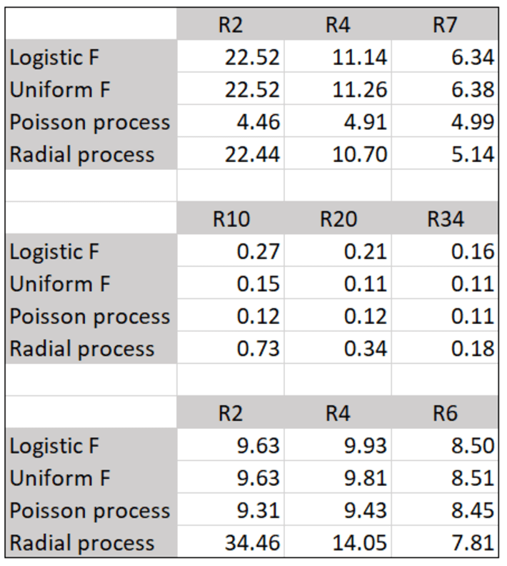
Table 1: Testing radiality
The first part of table 1 corresponds to the 2-D paired process pictured in figure 1, with a small value for the scaling factor s, and discussed in the first part of my article, here. The middle part is for the paired process too (figure 2 in first part of my article), but this time with a large s. The bottom part is for the unpaired process featured in figure 3 in this article, with a small s. The number Rx in table 1 is the ratio of the number of observed points in a circle B of radius x centered at the origin, divided by the area of that circle. The values in the table are thus estimates for E[N(B)]. Two Poisson-binomial processes with logistic and Uniform F are investigated, and compared with a stationary Poisson process and a radial process.
If the process is stationary, then the three numbers in any given row should be very similar. This is the case for unpaired Poisson-binomial (bottom part of table 1) and Poisson processes only. The radial process, as expected, has a huge concentration of points near the origin, as you can see in plot (f) in figure 3. This is just as true for the two paired Poisson-binomial processes with a small s (top part of table 1), though the higher point concentration this time is around the X-axis, rather than around the origin, and difficult to see to the naked eye. For the paired process, when s is large (middle part of table 1), the uneven point concentration is less noticeable: this is because as s gets larger and large, even the paired process approaches a stationary Poisson process.
Finally, the bottom part of the table shows stationarity for the unpaired process. Yet if you look at plot (d) in figure 3, where F is the uniform distribution, the points are almost evenly distributed and don’t look at all like a Poisson process. This is because s is small; this effect disappears when s gets bigger. This effect is barely visible to the naked eye in plot (a) in the same figure 3, corresponding to a logistic F. However, it is just as present and only detectable by doing further testing.
Better confidence intervals can be obtained by increasing the number of points, and this can be used to determine the optimum sample size.
5.6. Distributions related to the inverse or hidden process
Lets’ say that you observe points in a data set, but for each point, you don’t know which k created it. You are interested in retrieving the index k attached to each observed point x. In this case, x is fixed, and k, a function of x, is the unknow that you try to estimate. This is the inverse problem, sometimes called the hidden process, as in hidden Markov processes. Let’s L(x) be the discrete random variable equal to the index associated to x. What is the distribution of L(x)? It seems that P(L(x) = k) should be proportional to f( (x – k/λ) / s) where f is the symmetric density attached to F, and thus maximum when k is closest to λx. This has not been verified yet.
Another statistics of interest, K, also taking on integer values k (negative or positive) is the index of the point closest to the point X0, on the right-hand side on the real axis. The distribution of the arrival times T is the same as that of XK – X0. In other words,
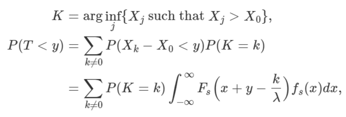
where Fs(z) = F(z/s) and fs(z), the density, is the derivative of Fs(z) with respect to z.
5.7. Convergence to Poisson point process
The Poisson-binomial process converges to a stationary point process of intensity λ when s tends to infinity. See theorem C and its proof, here. This is true regardless of the continuous distribution Fs, as long as Fs(x) = F(s/x), the density f exists and is continuous almost everywhere. It is also assumed that f is unimodal and centered at the origin. This result is true even for the Cauchy distribution, despite its thick tail and the fact that it does not have a mean nor a variance. In some sense, theorem C is some kind of central limit theorem (CLT) for this type of process. One that (unlike the standard CLT) even works for the Cauchy distribution. Not only that, but a Cauchy F provides faster convergence to a Poisson process (as s increases) than a uniform F does.
This may be generalized to indices (h, k) distributed on a random lattice. Such a random lattice could consist of the points of a Poisson-binomial process. The resulting process would be a compound Poisson-binomial process with two layers, similar to that displayed in Figure 4, except that the child process, rather than being radial, would be Poisson-binomial as the parent process.
Conclusion
We have introduced a special type of point process called Poisson-binomial, analyzed its properties and performed simulations to see the distributions of points that it generates, in one and two dimensions, as well as to make inference about its parameters. Statistics of interest include distance to nearest neighbors or interarrival times (some times called increments). Combined with radial processes, it can be used to model complex systems involving clustering, for instance the distribution of matter in the universe. Limiting cases are Poisson processes, and this may lead to what is probably the simplest definition of of stochastic, stationary Poisson point process. Our approach is not based on traditional statistical science, but instead on modern machine learning methodology. Some of the tests performed reveal strong patterns invisible to the naked eye.
Probably the biggest takeaway from this article is its tutorial value. It shows how to handle a machine learning problem involving the construction of a new model, from start to finish, with all the steps described at a high level, accessible to professionals with one year worth of academic training in quantitative fields. Numerous references are provided to help the interested reader dive into the technicalities. This article covers a large amount of concepts in a compact style: for instance, stationarity, isotropy, intensity function, paired and unpaired data, order statistics, hidden processes, interarrival times, point count distribution, model fitting, model-free confidence intervals, simulations, radial processes, renewal process, nearest neighbors, model identifiability, compound or hierarchical processes, Mahalanobis distance, rescaling, and more. It can be used as a general introduction to point processes. The accompanying spreadsheet has its own tutorial value, as it uses powerful Excel functions that are overlooked by many. Source code is also provided and included in the spreadsheet.
Other types of stochastic processes, more similar to infinite time series or Brownian motions, are described in my books Statistics: New Foundations, Toolbox, and Machine Learning Recipes (here) and Applied Stochastic Processes, Chaos Modeling, and Probabilistic Properties of Numeration Systems (here). The material discussed here will be part of a new book on stochastic processes that I am currently writing. The book will be available here.
To receive a weekly digest of our new articles, subscribe to our newsletter, here.
About the author: Vincent Granville is a machine learning scientist, author and publisher. He was the co-founder of Data Science Central (acquired by TechTarget) and most recently, founder of Machine Learning Recipes.