
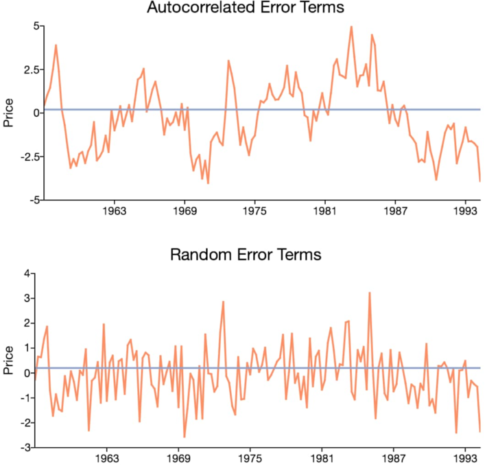
We describe here a methodology that applies to any statistical test, and illustrated in the context of assessing independence between successive observations in a data set. After reviewing a few standard approaches, we discuss our methodology, its benefits, and drawbacks. The data used here for illustration purposes, has known theoretical auto-correlations. Thus it can be used to benchmark various statistical tests. Our methodology also applies to data with high volatility, in particular, to time series models with undefined autocorrelations. Such models (see for instance Figure 1 in this article) are usually ignored by practitioners, despite their interesting properties.
Independence is a stronger concept than all autocorrelations being equal to zero. In particular, some functional non-linear relationships between successive data points may result in zero autocorrelation even though the observations exhibit strong auto-dependencies: a classic example is points randomly located on a circle centered at the origin; the correlation between the X and Y variables may be zero, but of course X and Y are not independent.
1. Testing for independence: classic methods
The most well known test is the Chi-Square test, see here. It is used to test independence in contingency tables or between two time series. In the latter case, it requires binning the data, and works only if each bin has enough observations, usually more than 5. Its exact statistic under the assumption of independence has a known distribution: Chi-Squared, itself well approximated by a normal distribution for moderately sized data sets, see here.
Another test is based on the Kolmogorov-Smirnov statistics. It is typically used to measure goodness of fit, but can be adapted to assess independence between two variables (or columns, in a data set). See here. Convergence to the exact distribution is slow. Our test described in section 2 is somewhat similar, but it is entirely data-driven, model free: our confidence intervals are based on re-sampling techniques, not on tabulated values of known statistical distributions. Our test was first discussed in section 2.3 of a previous article entitled New Tests of Randomness and Independence for Sequences of Observations, and available here. In section 2 of this article, a better and simplified version is presented, suitable for big data. In addition, we discuss how to build confidence intervals, in a simple way that will appeal to machine learning professionals.
Finally, rather than testing for independence in successive observations (say, a time series) one can look at the square of the observed autocorrelations of lag-1, lag-2 and so on, up to lag-k (say k = 10). The absence of autocorrelations does not imply independence, but this test is easier to perform than a full independence test. The Ljung-Box and the Box-Pierce tests are the most popular ones used in this context, with Ljung-Box converging faster to the limiting (asymptotic) Chi-Squared distribution of the test statistic, as the sample size increases. See here.
2. Our Test
The data consists of a time series x1, x2, …, xn. We want to test whether successive observations are independent or not, that is, whether x1, x2, …, xn-1 and x2, x3, …, xn are independent or not. It can be generalized to a broader test of independence (see section 2.3 here) or to bivariate observations: x1, x2, …, xn versus y1, y2, …, yn. For the sake of simplicity, we assume that the observations are in [0, 1].
2.1. Step #1: Computing some probabilities
The first step to perform the test, consists in computing the following statistics:
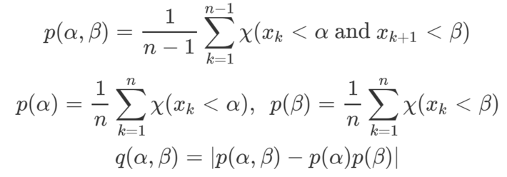
for N vectors (α, β)‘s, where α, β are randomly sampled or equally spaced values in [0, 1], and Ï is the indicator function: Ï(A) = 1 if A is true, otherwise Ï(A) = 0. The idea behind the test is intuitive: if q(α, β) is statistically different from zero for one or more of the randomly chosen (α, β)’s, then successive observations can not possibly be independent, in other words, xk and xk+1 are not independent.
In practice, I chose N = 100 vectors (α, β) evenly distributed on the unit square [0, 1] x [0, 1], assuming that the xk‘s take values in [0, 1] and that n is much larger than N, say n = 25 N.
2.2. Step #2: The statistic associated with the test
Two natural statistics for the test are
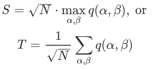
The first one S, once standardized, should asymptotically have a Kolmogorov-Smirnov distribution. The second one T, once standardized, should asymptotically have a normal distribution, despite the fact that the various q(α, β)’s are never independent. However, we do not care about the theoretical (asymptotic) distribution, thus moving away from the classic statistical approach. We use a methodology that is typical of machine learning, and described in section 2.3.
Nevertheless, the principle is the same in both cases: the higher the value of S or T computed on the data set, the most likely we must reject the assumption of independence. Among the two statistics, T has less volatility than S, and may be preferred. But S is better at detecting very small departures from independence.
2.3. Step #3: Assessing statistical significance
The technique described here is very generic, intuitive, and simple. It applies to any statistical test of hypotheses, not just for testing independence. It is somewhat similar to cross-validation. It consists or reshuffling the observations in various ways (see the resampling entry in Wikipedia to see how it actually works) and compute S (or T) for each of the 10 different reshuffled time series. After reshuffling, one would assume that any serial, pairwise independence has been lost, and thus you get an idea of the distribution of S (or T) in case of independence. Now compute S on the original time series. Is it higher than the 10 values you computed on the reshuffled time series? If yes, you have a 90% chance that the original time series exhibits serial, pairwise dependency.
A better but more complicated method consists of computing the empirical distribution of the xk‘s, then generate 10 n independent deviates with that distribution. This constitutes 10 time series, each with n independent observations. Compute S for each of these time series, and compare with the value of S computed on the original time series. If the value computed on the original time series is higher, then you have a 90% chance that the original time series exhibits serial, pairwise dependency. This is the preferred method if the original time series has strong, long-range autocorrelations.
2.4. Test data set and results
I tested the methodology on an artificial data set (a discrete dynamical system) created as follows: x1 = log(2) and xn+1 = b xn – INT(b xn). Here b is an integer larger than 1, and INT is the integer part function. The data generated behaves like any real time series, and has the following properties.
- The theoretical distribution of the xk‘s is uniform on [0, 1]
- The lag-k autocorrelation is known and equal to 1 / b^k (b at power k)
It is thus easy to test for independence and to benchmark various statistical tests: the larger b, the closer we are to independence. With a pseudo-random number generator, one can generate a time series consisting of independently and identically distributed deviates, with a uniform distribution on [0, 1], to check the distribution of S (or T) and its expectation, in case of true independence, and compare it with values of S (or T) computed on the artificial data, using various values of b. In this test with N = 100 n = 2500, b = 4, (corresponding to an autocorrelation of 0.25) the value of S is 6 times larger than the one obtained for full independence. For b = 8, (corresponding to an autocorrelation of 0.125), S is 3 times larger than the one obtained for full independence. This validates the test described here at least on this kind of dataset, as it correctly detects lack of independence by yielding abnormally high values of T when the independence assumption is violated.
Note: Another interesting feature of the dataset used here is this: using b^k (b at power k) instead of b, is equivalent to checking lag-k independence, that is, independence between x1, x2, … and x1+k, x2+k, … in the original time series corresponding to b. The reason being that in the original series (corresponding to b), we have xn+k = b^k xn – INT(b^k xn).
To receive a weekly digest of our new articles, subscribe to our newsletter, here.
About the author: Vincent Granville is a data science pioneer, mathematician, book author (Wiley), patent owner, former post-doc at Cambridge University, former VC-funded executive, with 20+ years of corporate experience including CNET, NBC, Visa, Wells Fargo, Microsoft, eBay. Vincent is also self-publisher at DataShaping.com, and founded and co-founded a few start-ups, including one with a successful exit (Data Science Central acquired by Tech Target). You can access Vincent’s articles and books, here.