
We investigate a large class of auto-correlated, stationary time series, proposing a new statistical test to measure departure from the base model, known as Brownian motion. We also discuss a methodology to deconstruct these time series, in order to identify the root mechanism that generates the observations. The time series studied here can be discrete or continuous in time, they can have various degrees of smoothness (typically measured using the Hurst exponent) as well as long-range or short-range correlations between successive values. Applications are numerous, and we focus here on a case study arising from some interesting number theory problem. In particular, we show that one of the times series investigated in my article on randomness theory [see here, read section 4.1.(c)] is not Brownian despite the appearance. It has important implications regarding the problem in question. Applied to finance or economics, it makes the difference between an efficient market, and one that can be gamed.
This article it accessible to a large audience, thanks to its tutorial style, illustrations, and easily replicable simulations. Nevertheless, we discuss modern, advanced, and state-of-the-art concepts. This is an area of active research.
1. Introduction and time series deconstruction
We are dealing with a series of N observations or events denoted as z(1), …, z(N) and indexed by time. The respective times of arrival are denoted as T(1), …, T(N). Events are equally spaced in time, and typically, N is large while time intervals are small, thus providing a good approximation to a time-continuous process. The time series discussed here are assumed to have stationary increments with unit variance and zero mean. We will define what this means exactly when needed.
1.1. Example
The picture below shows typical examples of the time series that we are dealing with in this article. The X-axis represents the time. These are discrete approximations of time-continuous series found in many contexts, in particular in finance.
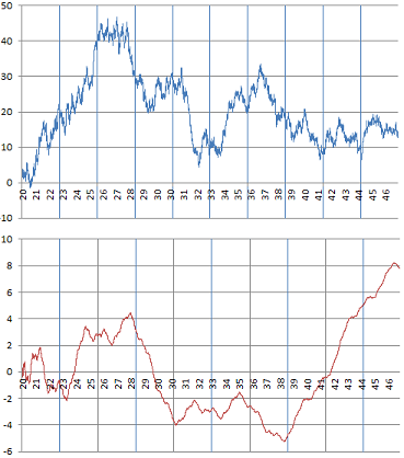
Smooth (bottom) versus rugged time series (top)
Interestingly, these two examples come from number theory, and are studied later in this article. In each case, it consists of 22,000 observations. The chart at the top is a classic example of a Brownian motion, while the one at the bottom exhibits long-range auto-correlations not found in traditional Brownian motions. The statistical tests discussed in section 2 help assess which type of time series we are dealing with. .
1.2. Deconstructing time series
The observed time series considered here are typically the result of a cumulative process. The parent process { y(n) } causing the pattern usually results (but not always as we shall see) in { z(n) } being a Brownian motion or a fractional Brownian motion. The parent process, sometimes called differential process, is defined as follows:

The square root factors in the above formula are needed, as increments z(n) – z(n – 1) are very small, since { z(n) } mimics a time-continuous process. For instance, in the above figure, we have 750 observations in a time interval of length 1. And indeed, if you do the reverse operation, starting with the parent process — consisting (say) of independent and identically distributed random variables with mean 0 and variance 1 — then
The square root factor is clearly mandatory here, by virtue of the central limit theorem, to keep the variance finite and non-zero in { z(n) }. For details, see chapter 1 in my book on applied stochastic processes.
Note:
If your observed { z(n) } is stationary, proceed as follows. Shift the time axis (that is, shift the T(n) values) so that the new origin is far in the future. This is implemented and illustrated in my spreadsheet (shared later in this article) via the offset parameter, and it fixes issues near the origin. Indeed, if { z(n) } is stationary, then time location does no matter as far as probabilistic properties are concerned, because of the very definition of stationarity. By doing so, the parent process { y(n) } is also (almost) stationary.
1.3. Correlations, Fractional Brownian motions
The traditional setting consists of { y(n) } being a white noise, that is, a sequence of independent and identically distributed random variables with mean 0 and variance 1 in this case. The resulting time-continuous limit of { z(n) } is then called a Brownian motion. In most cases investigated here, the y(n)’s are not independent and exhibit auto-correlations. The resulting process is then called a fractional Brownian motion. And in some cases, { y(n) } may not even be stationary. We will show what happens then.
The stronger the long-range correlations in { y(n) }, the smoother { z(n) } looks like. The degree of smoothness is usually measured using the Hurst exponent, described in the next section.
2. Smoothness, Hurst exponent, and Brownian test
The traditional and simple metric to measure the smoothness in your data is called the detrending moving average, and it is abbreviated as DMA. It is the mean square error between your observations and its various moving averages of order m = 1, 2, 3, and so on. The exact definition can be found in this article (Statistical test for fractional Brownian motion based on detrending moving, by Grzegorz Sikoraa, 2018, see section 2). Other criteria are also used, such as FA and DFA. A comparison of these metrics can be found in this article (Comparing the performance of FA, DFA and DMA using different synthetic long-range correlated time series, by Ying-Hui Shao et al., 2018). DMA, along with other metrics, are used in our computations.
With the notation DMA(m) to emphasize the fact that it depends on m, we have this well-known result:
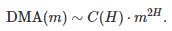
This is an asymptotic result, meaning that it becomes more accurate as m grows to infinity. The constant H is known as the Hurst exponent. See here (section 2) for details. H takes on values between 0 and 1, with H = 1/2 corresponding to the Brownian motion (see also here.) Higher values correspond to smoother time series, and lower values to more rugged data.
Let’s N be the number of observations in your time series. We used N = 22,000 in all our examples, and typically, m of the order SQRT(N). The above asymptotic result is not applicable in our context, and we use a slightly different methodology.
2.1. Our Brownian tests of hypothesis
Testing the Brownian character of a time series is typically done using the above formula with the Hurst exponent. See here and here for details. Our approach here is different, as we are more interested in small-range and mid-range correlations, than in long-range ones. We use the notation S(N, m) instead of DMA(m), since this metric also depends on your sample size N.
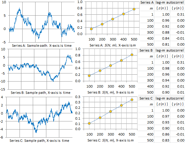
We performed two types of tests. The first one is based on S(N, m), and we used m = 100, 200, up to 500. We used the correlation R between { S(N, m) } and { m } computed on these 5 values of m, with N = 22,000. Since the correlation is very close to 1 in all examples, the actual test statistic is -log(1 – R). Its distribution can be empirically computed by simulations. The second test is based on auto-correlations of lag m, with m = 1, 100, 200, 300, 400 and 500, both for the observations { z(n) } and the deconstructed time series { y(n) }. The result with detailed computations, using 6 time series A, B, C, D, E, F, are available in my spreadsheet in section 2.2.
2.2. Data
We tested the methodology on different types of time series. The results are illustrated in the pictures below, and replicable using my spreadsheet. The time series { z(n) } were constructed as follows:
- Create a base process { x(n) }.
- Standardize { x(n) } so that its mean and variance become 0 and 1 respectively. The resulting sequence is { y(n) }.
- Create the cumulative process { z(n) } using the formula in section 1.2.
The time T(n) was set to T(n) = 600 + n / 750. That’s what makes the series { z(n) } look like continuous in time.
The six time series (simulations) investigated here are constructed as follows. They are also pictured in section 3.1. Here INT is the integer part function.
- Series A: Use x(n + 1) = bx(n) – INT(bx(n)) with x(1) = log 2 and b = (1 + SQRT(5)) / 2.
- Series B: Use x(n + 1) = bx(n) – INT(bx(n)) with x(1) = Pi / 4 and b = (1 + SQRT(5)) / 2.
- Series C: Here x(n) is a Bernouilli deviate of parameter 1/2. The x(n)’s are independent.
- Series D: Use x(n + 1) = b + x(n) – INT(b + x(n)) with x(1) = 1 and b = SQRT(2). In addition, use z‘(n) = z(n) – SQRT(n)/2, rather than the standard z(n).
- Series E: Use x(n + 1) = b + x(n) – INT(b + x(n)) with x(1) = log 2 and b = 16 Pi. In addition, use z‘(n) defined by z’(n + 1 ) = z‘(n) + z(n + 1)/(T(n))^3, with z‘(1) = z(1) and T(1) =24, rather than the standard z(n).
- Series F: Use x(n + 1) = b + x(n) – INT(b + x(n)) with x(1) = 0 and b = (1 + SQRT(5)) / 2.
Series A and B are generated by a b-process, while series D, E, and F are generated by a perfect process. The purpose of this study was to compare b-processes with perfect processes, and their ability to generate Brownian motions of fractional Brownian motions. Perfect processes and b-processes were introduced in my article on the theory of randomness, see here. Series D is actually pictured in section 4.1.(c) in that article. Series C corresponds to the classic Brownian motion.
The data and computations are available in my spreadsheet, here. Both columns D and I represent the same exact { y(n) } in the spreadsheet. But column D is used to build { z(n) }, while column I assumes that you only observe { z(n) } and must compute { y(n) } from scratch, by deconstructing { z(n) }.
3. Results and conclusions
In this section, we summarize our findings. Many illustrations are provided.
3.1. Charts and interpretation
The first three series A, B, C in our picture below feature processes that behave pretty much like Brownian motions, with an Hurst exponent H equal or close to 1/2. Series A and B are two realizations of the exact same processes, as b is identical in both cases. Series C illustrates a perfect Brownian motion, with H = 1/2.
Note that the auto-correlations in the deconstructed time series { y(n) } rapidly drop to 0, while the correlations in { z(n) } are very high, but slowly drop to a value between 0.80 and 0.90 when m = 500. As a result, S(N, m), as a function of m, is a perfect straight line (m is the order of the moving average; N = 22,000 is the total number of observations.)
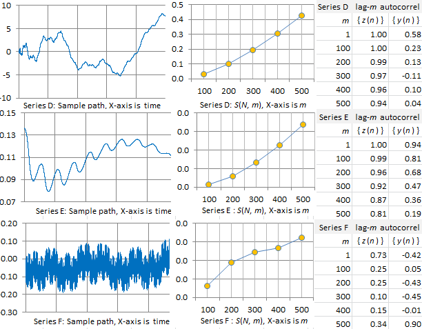
Time series D, E, and F, pictured below, behave very differently from A, B, and C. Series D exhibits very high auto-correlations in { z(n) } while auto-correlations in { y(n) } slowly drop to 0. It is smoother than A, B, and C. As a result, S(N, m), as a function of m, is no longer a straight line: it is now a convex function. If this was a financial time series, it would correspond to a non efficient market. So the statistical tests described in section 2 can be use to test market efficiency.
The smoothness is even more pronounced in series E. In this case, auto-correlations in { y(n) } are long-range and do not drop to zero. Series F, to the contrary, is very rugged. Auto-correlations in { z(n) } are lower than in the other examples, and S(N, m) is now mostly concave. There are still long-range auto-correlations if you look at { y(n) }. We are dealing with a mixture of smoothness and bumpiness, though the smooth part is not visible with the naked eye. The rugged part also shows up in the first half of the S(N, m) curve, which is concave, while the smooth part shows up in the second half of the S(N, m) curve, which is convex.
3.2. Conclusions
We have explored four types of time series, and characterized them using auto-correlation indicators:
- Brownian-like with very short-range auto-correlations in the deconstructed time series { y(n) }. Examples: series A and B.
- Brownian for series C, with no auto-correlation in the deconstructed time series { y(n) }.
- Smooth, fractional Brownian-like for series D (in series E, { y(n) } is not stationary, so it is not Brownian at all).
- Rugged, fractional Brownian-like for series E
The tests presented here can be integrated in a Python library. The initial purpose was to compare b-processes (series A and B) with perfect processes (series D, E and F). These two processes have been found here to be very different. Indeed, perfect processes are so peculiar that the standard division by SQRT(n) in the construction of { z(n) } [section 1.2.] does not work. Factors other than SQRT(n) must be used, and even then, the final time series { z(n) } is not a perfect Brownian motion, not even close: it usually has a smooth component and long-range auto-correlations in { y(n) }. This makes perfect processes less attractive than b-processes, for use in cryptographic applications. But more attractive, to model inefficient markets or less than perfect randomness.
To not miss this type of content in the future, subscribe to our newsletter. For related articles from the same author, click here or visit www.VincentGranville.com. Follow me on on LinkedIn, or visit my old web page here.
DSC Resources
- A Plethora of Original, Not Well-Known Statistical Tests
- Free Book and Resources for DSC Members
- New Perspectives on Statistical Distributions and Deep Learning
- Time series, Growth Modeling and Data Science Wizardy
- Statistical Concepts Explained in Simple English
- Machine Learning Concepts Explained in One Picture
- Comprehensive Repository of Data Science and ML Resources
- Advanced Machine Learning with Basic Excel
- Difference between ML, Data Science, AI, Deep Learning, and Statistics
- Selected Business Analytics, Data Science and ML articles
- How to Automatically Determine the Number of Clusters in your Data
- Fascinating New Results in the Theory of Randomness
- Hire a Data Scientist | Search DSC | Find a Job
- Post a Blog | Forum Questions