
In this article, we discuss a general framework to drastically reduce the influence of outliers in most contexts. It applies to problems such as clustering (finding centroids,) regression, measuring correlation or R-Squared, and many more. We will focus on the centroid problem here, as it is very similar and generalizes easily to solving a linear regression. The correlation / R-Squared issue was discussed in an earlier article and involves only a change of formula. Clustering and regression are more complex problems involving iterative algorithms.
This article also features interesting material for future data scientists, such as
- Several outlier detection techniques
- How to display contour maps and images corresponding to an intensity function or heatmap, in R (in just a few lines of code, and very easy to understand) — see section 5 below
- How to produce data sets that simulate clustering structures or other patterns
- Distribution of arrival times for successive records in a time series
1. General Framework
We discuss replacing techniques used by statisticians, based on optimizing traditional L^2 metrics such as variance, by techniques based on L^p metrics, which are more robust when 1 < p < 2. The case p = 2 corresponds to the traditional framework, Throughout the article, p is referred to as the power. The regression and centroid problems being equivalent, we focus here on finding a centroid using the L^p criterion (denoted as H), and we show how to modify it for regression problems. Illustrations are in a 2-dimensional space (d = 2) but easily generalize to any dimension, especially as we are not using any matrix inversions to solve the problem.
Finding a robust centroid
The focus here is on finding the point that minimizes the sum of the “distances” to n points in a d-dimensional space, called centroid or center, especially in the presence of outliers.
The sum of “distances” between an arbitrary point (u, v) and a set S = { (x(1), y(1)) … (x(n), y(n)) } of n points is defined as follows:
H((u,v), S; p) = SUM{ (e + |x(k) – u|)^p + (e + |y(k) – v|^p } / n,
where e is a very small positive quantity, equal to zero unless p is negative; the sum is over k = 1,…,n.
The function H has one parameter p called power, and when p = 2, we are facing the traditional problem of finding the centroid of a cloud of points: in this case, the solution is the classic average of the n points. This solution is notoriously sensitive to outliers. When 1 < p < 2, we get get a more stable solution, less sensitive to outliers, yet when n is large (> 20) and the proportion of outliers is small (by definition it is always small!), the solution is pretty much the same regardless of p (assuming 1 < p < 3).
In short, what we are trying to accomplish here is to build a robust measure of centrality in any dimension, just like the median is a robust measure of centrality in dimension d = 1.
Generalization to linear regression problems
The same methodology can be used for regression. With 2 parameters u and v as in Y = u X + v, the function H becomes
H((u,v), S; p) = SUM{ (e + |y(k) – u * x(k) – v|)^p } / n,
again with e = 0 if p > 0. It generalizes easily to more than 2 parameters u, v.
General outlier detection techniques
Our proposed method smooths out the impact of outliers rather than detecting them. For outlier detection and removal, you can use one of these methods:
- Using traditional centrality measures and eliminating the points farthest away from the center, then re-computing the center and proceeding iteratively with eliminating newly found outliers until stability is reached.
- Using the median both for the x- and y-coordinates, rather than the average.
- The leaving-one-out technique consists of computing the convex hull of your data set S, then removing one point at a time, and re-computing the convex hull after removing the point in question. The point resulting in the largest loss of volume in the convex hull, when removed, corresponds to the strongest outlier.
- Identifying points of lowest density using density estimation techniques.
- Nearest neighbor distances: a point far away from its nearest neighbors is potentially an outlier. Compute all nearest neighbor distances and look for the most extremes.
Another way to attenuate the impact of outliers is to use a weighted sum for H, that is (in the case of the regression problem) to use the formula
H((u,v), S; p) = SUM{ q(k) * (e + |y(k) – u * x(k) – v|)^p } / n,
where q(k) is the weight attached to point k, with SUM{ q(k) } = 1. In this case, a point with low density is assigned a smaller weight.
To read more about outlier detection, click here.
A related physics problem
When p < 0, and especially when p = -2, maximizing or minimizing H becomes an interesting physics problem of optimizing a potential H. The centroid problem is now equivalent to finding the point of maximum or minimum light, sound, radioactivity, or heat intensity, in the presence of an energy field produced by n energy source points. Both problems are closely related and use the same algorithm to find solutions.
However, the case p < 0 has no practical value to data scientists or statisticians (as far as I know) and it presents the following challenges:
- If (u, v) is a point of S and p < 0, then H((u,v), S; p) is infinite: we have singularities. This is dealt with by introducing the very small constant e > 0 in the definition of H. This quantity is used to address the fact that in the real world, no source of energy is a point with an area of zero and positive (but finite) intensity. This artifact of physics models is discussed here.
- If you want to minimize H, there will be an infinite number of solutions, all located far outside the cloud of points S. Think about finding the point in the universe that receives the least amount of light from the solar system. So typically one is interested in finding a maximum, not a minimum (unless you put constraints on the solution, such as being located inside the convex hull of S.)
- Even if searching for a maximum of H, the convergence may be slow and chaotic, as you can end up with several maxima (H is no longer a nice, smooth curve when p < 0.)
2. Algorithm to find centroid when p > 1
There are many algorithms available to solve this type of mathematical optimization problem. A popular class of algorithms is based on gradient descent and boosting. Here however, we use what is possibly the simplest algorithm. Why? For two reasons. First it is very easy to understand, still leads to some interesting research, is easy to replicate, and keep the focus on the concepts and the results associated with the centroids, rather than on a specific implementation. Second, with modern computers (even on my 10 years old laptop) the computing power is big enough that naive algorithms perform well. If you are OK with getting results accurate to two or three digits — and in real life, many data sets, even web analytics measured using two different sources, do not have higher accuracy — then a rudimentary algorithm is enough.
So here I used rudimentary Monte-Carlo to find the centroids. However, in higher dimensions (d > 3) be careful about the curse of dimensionality. Note that when p < 0, Monte Carlo is not that bad, as it allows you to visit and circle around several local minima. It is also easy to deploy in a Map-Reduce environment (Hadoop.) The algorithm is actually so simple that there is no need to describe it: the short, easy-to-read source code below (Perl) speaks for itself.
Source code to generate points and compute centroid, using Monte Carlo
Notes about the source code:
- The first n points in the output file centroid.txt are the simulated sample points (random deviates on [0, 1] x [0, 1]. The last point is the centroid computed on the sample points.
- Note that $seed (first line of code) is used to initiate the random generator and for reproducibility purposes. Also, I noticed that a value of $seed lower than 1,000 causes the first random deviate generated to be biased (unusually small.)
- The variable $sum stores, at each iteration $iter, the value of the function H that we try to minimize.
Below is the source code.
$seed=1000;
srand($seed);
$n=100;
open(OUT,”>centroid.txt”);
for ($k=0; $k<$n; $k++) {
$x[$k]=rand();
$y[$k]=rand();
print OUT “$x[$k]\t$y[$k]\n”; # one of the n simulated points
}
$power = 1.25; # corresponds to p (the power) in the article
$niter = 200000;
$eps = 0.00001; # the “e” in the H function (see article)
$min=99999999;
for ($iter=0; $iter<$niter; $iter++) {
$u=rand();
$v=rand();
$sum=0;
for ($k=0; $k<$n; $k++) {
$dist=exp($power*log($eps+abs($x[$k]-$u)))+exp($power*log($eps+abs($y[$k]-$v)));
$sum+=$dist;
}
$sum = $sum/$n;
if ($sum < $min) {
$min=$sum;
$x_centroid=$u;
$y_centroid=$v;
}
}
print OUT “$x_centroid\t$y_centroid\n”;
close(OUT);
Generating point clouds with simulation
In the few lines of the source code (above), we generated points randomly distributed in the unit square [0, 1] x [0, 1] . In order to simulate outliers or more complicated distributions that represent real-life problems, one has to use more sophisticated techniques. Click here to get the source code to easily generate a cluster structure (illustrated in figure 1 below).
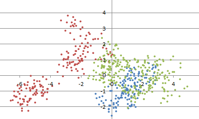
Figure 1: example of simulated clustered point cloud
More complex simulations (random clusters evolving over time) can be found here. Some simple stochastic processes can be simulated by first simulating random points (called centers) uniformly distributed in a rectangle, then, around each center, simulating a random number of points radially distributed around each center. Other techniques involve thinning, that is, removing some points afver over-si,ulating a large number of points.
3. Examples and results
A few examples are provided in the next section to validate the methodology. In this section, rather than validation, we focus on showing its usefulness when 0 em>p < 2, compared to the traditional solution consisting of using p = 2, found in all statistical packages. Note that the traditional solution (p = 2) was designed not out of practical considerations such as robustness, but because of its ease of computation at a time when computers did not exist, and data sets were manually built.
To test the methodology, we created various data sets, introduced outliers, and computed the centroid using different values of p. The example shown in Figure 2, consisting of five points (bottom left) plus an outlier (top right) illustrates the performance. The six data points are in blue. The centroids, computed for p = 0.75, 1.00, 1.25, 1.50, 1.75 and 2.00, are in red. The rightmost centroid corresponds to p = 2: this is the classic centroid. Due to the outlier, it is located outside the convex hull of the five remaining points, which is awkward. The leftmost centroid corresponds to p = 0.75 and is very close to the traditional centroid obtained after removing the outlier. I also tried the values p = 0.25 and p = 0.50, but failed to obtain convergence to a unique solution after 200,000 iterations.
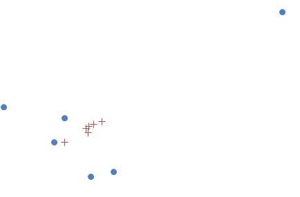
Figure 2: the blue dots represent the data points, the red + the centroid (computed for 6 values of p)
Note that the scale does not matter. Finally, using p < 2 does not fully get rid of the influence of the outlier, but instead, it reduces its impact when computing the centroid. To completely get rid of the outliers, a methodology using medians computed for the x- and y-axis, is more efficient.
If you are wondering how to produce a scatter plot in Excel with two data sets (points and centroids) as in Figure 2, click here for instructions: it is easier than you think.
4. Convergence of the algorithm
Figure 3 shows the speed of convergence of the algorithm, using the same source code as in section 2 with p = 1.4. So you can replicate these results. In this case, the data set S consists of n = 100 points randomly (uniformly) distributed on [0, 1] x [0, 1].
About 10,000 iterations in the outer loop are needed to reach two digits of accuracy, and this requires a tiny fraction of a second to compute. This “10,000 iterations” is actually a rule of thumb for any Monte-Carlo algorithm used to find an optimum with two correct digits. Note that in Figure 3, only iterations providing an improvement over the current approximation of the centroid — that is, iterations where the value of H is smaller than those computed in all previous iterations — are displayed. A potential research topic is to investigate the asymptotic behavior of these “records”, in the example below occurring at iterations 0, 4, 12, 44, 109, 156, and so on.
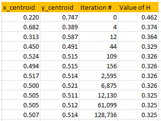
Figure 3: convergence of the algorithm (p = 1.4)
Since the n = 100 simulated points were randomly (uniformly) distributed in [0, 1] x [0, 1] it is no surprise that the centroid found by the algorithm, after convergence, is very close to (0.5, 0.5).
Indeed, we tried values of p equally spaced between 1.25 and 3.50, and in each case, the centroid found was also very close to (0.5, 0.5), see Figure 4. That includes the special case p = 2 (it is located somewhere on the chart below) corresponding to the classic average of the n points. Note that here, no outliers were introduced in the simulations.
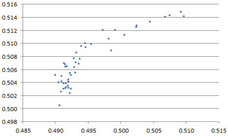
Figure 4: x- and y-coordinates of centroid, obtained with various values of p
5. Interesting Contour Maps
The following contour maps in Figure 5, produced with the contour function in R, show that as p gets closer to 0, the function H becomes more chaotic, exhibiting local minima. These charts were produced using a data set S consisting of n = 20 points randomly (uniformly) distributed on [0, 1] x [0, 1]. It is interesting to notice that, despite the random distribution of the n points, strong patterns emerge when p < 1 (the statistical significance of these patterns is weak though.).
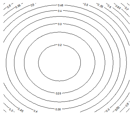
Figure 5A: Contour map for H, with n = 20 and p =2
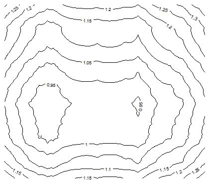
Figure 5B: Contour map for H, with n = 20 and p = 0.50
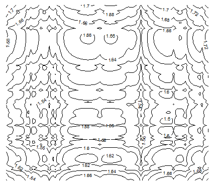
Figure 5C: Contour map for H, with n = 20 and p = 0.15
You can also plot images of H, using the function image in R with a gray palette with 300 levels of grey, using the command image(z, col = gray.colors(300)) where z is an m x m matrix (in R) representing values of H computed at m x m locations (here m = 100 and n = 20.)
The source code (in R) looks like this:
data<-read.table(“c:/vincentg/math2r.txt”,header=TRUE)
w<-data$H
z <- matrix(w, nrow = 100, ncol = 100, byrow = TRUE)
image(z, col = gray.colors(300))
Here the file math2r.txt stores the m x m values of H sequentially in a one-column text file, row after row. The first row is the header (equal to H.) Note that in order to produce Figure 5, we used contour(z) rather than image(z, col = gray.colors(300)). In Figure 6 we actually used the function image to display H values for p = 0.5: low values of H (corresponding to proximity to centroid) are in a darker color, and unlike the case p = 2, you can notice multiple local minima. Figure 6 is based on the same data as Figure 5B. The source code to produce the input file math2r.txt can be found here..

Figure 6: H values displayed in an image using R (n = 20 and p = 0.5)
As a bonus, below is Figure 7 corresponding to p = -2, which interestingly is very similar to p = 0.5 (see Figure 5B.) This value of p has tremendous applications in physics, as it corresponds to the inverse-square law.
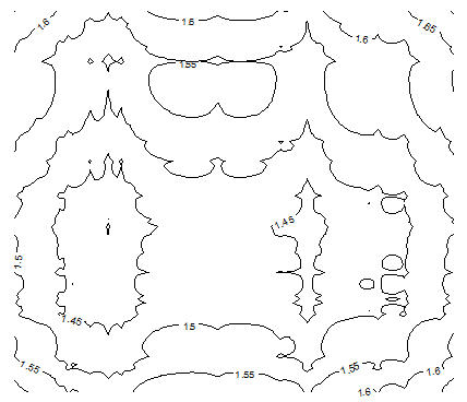
Figure 7: this time with p=-2
Top DSC Resources
- Article: Difference between Machine Learning, Data Science, AI, Deep Learnin…
- Article: What is Data Science? 24 Fundamental Articles Answering This Question
- Article: Hitchhiker’s Guide to Data Science, Machine Learning, R, Python
- Tutorial: Data Science Cheat Sheet
- Tutorial: How to Become a Data Scientist – On Your Own
- Categories: Data Science – Machine Learning – AI – IoT – Deep Learning
- Tools: Hadoop – DataViZ – Python – R – SQL – Excel
- Techniques: Clustering – Regression – SVM – Neural Nets – Ensembles – Decision Trees
- Links: Cheat Sheets – Books – Events – Webinars – Tutorials – Training – News – Jobs
- Links: Announcements – Salary Surveys – Data Sets – Certification – RSS Feeds – About Us
- Newsletter: Sign-up – Past Editions – Members-Only Section – Content Search – For Bloggers
- DSC on: Ning – Twitter – LinkedIn – Facebook – GooglePlus
Follow us on Twitter: @DataScienceCtrl | @AnalyticBridge