
When dealing with time series, the first step consists in isolating trends and periodicites. Once this is done, we are left with a normalized time series, and studying the auto-correlation structure is the next step, called model fitting. The purpose is to check whether the underlying data follows some well known stochastic process with a similar auto-correlation structure, such as ARMA processes, using tools such as Box and Jenkins. Once a fit with a specific model is found, model parameters can be estimated and used to make predictions.
A deeper investigation consists in isolating the auto-correlations to see whether the remaining values, once decorrelated, behave like white noise, or not. If departure from white noise is found (using a few tests of randomness), then it means that the time series in question exhibits unusual patterns not explained by trends, seasonality or auto correlations. This can be useful knowledge in some contexts such as high frequency trading, random number generation, cryptography or cyber-security. The analysis of decorrelated residuals can also help identify change points and instances of slope changes in time series, or reveal otherwise undetected outliers.
So, how does one remove auto-correlations in a time series?
One of the easiest solution consists at looking at deltas between successive values, after normalization.. Chances are that the auto-correlations in the time series of differences X(t) – X(t-1) are much smaller (in absolute value) than the auto-correlations in the original time series X(t). In the particular case of true random walks (see Figure 1), auto-correlations are extremely high, while auto-correlations measured on the differences are very close to zero. So if you compute the first order auto-correlation on the differences, and find it to be statistically different from zero, then you know that you are not dealing with a random walk, and thus your assumption that the data behaves like a random walk is wrong.
Auto correlations are computed as follows. Let X = X(t), X(t-1), … be the original time series, Y = X(t-1), X(t-2), … be the lag-1 time series, and Z = X(t-2), X(t-3), … be the lag-2 time series. The following easily generalizes to lag-3, lag-4 and so on. The first order correlation is defined as correl(X, Y) and the second order correlation is defined as correl(X, Z). Auto-correlations decrease to zero in absolute value, as the order increases.
While there is little literature on decorrelating time series, the problem is identical to finding principal components among X, Y, Z and so on, and the linear algebra framework used in PCA can also be used to decorrelate time series, just like PCA is used to decorrelate variables in a traditional regression problem. The idea is to replace X(t) by (say) X(t) + a X(t-1) + b X(t-2) and choose the coefficients a and b to minimize the absolute value of the first-order auto-correlation on the new series. However, we favor easier but more robust methods — for instance looking at the deltas X(t) – X(t-1) — as these methods are not subject to over-fitting yet provide nearly as accurate results as exact methods.
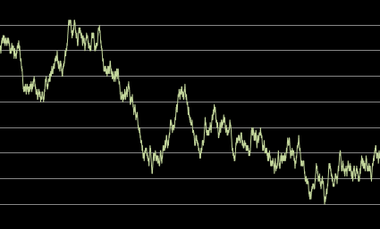
Figure 1: Auto-correlations in random walks are always close to +1
Example
In figure 2, we simulated an auto-correlated time series as follows: X(t+1) = X(t) + U(t) where U(t) are independent uniform deviates on [-0.5, 0.5]. The resulting time series is a random walk (with no trend and no periodicity) with a lag-1 auto-correlation of 0.99 when measured on the first 100 observations. The lag-1 auto-correlation measured on the deltas (blue curve) of decorrelated observations is 0.00.
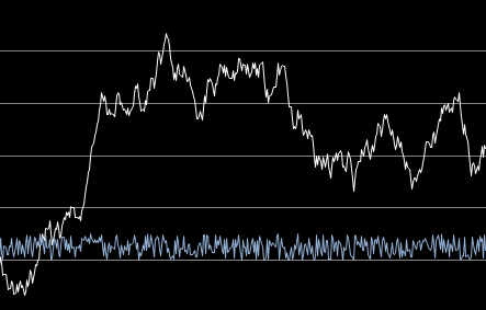
Figure 2: original (white) and decorrelated (blue) time series
Top DSC Resources
- Article: Difference between Machine Learning, Data Science, AI, Deep Learnin…
- Article: What is Data Science? 24 Fundamental Articles Answering This Question
- Article: Hitchhiker’s Guide to Data Science, Machine Learning, R, Python
- Tutorial: Data Science Cheat Sheet
- Tutorial: How to Become a Data Scientist – On Your Own
- Tutorial: State-of-the-Art Machine Learning Automation with HDT
- Categories: Data Science – Machine Learning – AI – IoT – Deep Learning
- Tools: Hadoop – DataViZ – Python – R – SQL – Excel
- Techniques: Clustering – Regression – SVM – Neural Nets – Ensembles – Decision Trees
- Links: Cheat Sheets – Books – Events – Webinars – Tutorials – Training – News – Jobs
- Links: Announcements – Salary Surveys – Data Sets – Certification – RSS Feeds – About Us
- Newsletter: Sign-up – Past Editions – Members-Only Section – Content Search – For Bloggers
- DSC on: Ning – Twitter – LinkedIn – Facebook – GooglePlus
Follow us on Twitter: @DataScienceCtrl | @AnalyticBridge