
Most of the articles on extreme events are focusing on the extreme values. Very little has been written about the arrival times of these events. This article fills the gap.
We are interested here in the distribution of arrival times of successive records in a time series, with potential applications to global warming assessment, sport analytics, or high frequency trading. The purpose here is to discover what the distribution of these arrival times is, in absence of any trends or auto-correlations, for instance to check if the global warming hypothesis is compatible with temperature data obtained over the last 200 years. In particular it can be used to detect subtle changes that are barely perceptible yet have a strong statistical significance. Examples of questions of interest are:
- How likely is it that 2016 was the warmest year on record, followed by 2015, then by 2014, then by 2013?
- How likely is it, in 200 years worth of observations, to observe four successive records four years in a row, at any time during the 200 years in question?
The answer to the first question is that it is very unlikely to happen just by chance..
Despite the relative simplicity of the concepts discussed here, and their great usefulness in practice, none of the material below is found in any statistics textbook, as far as I know. It would be good material to add to any statistics curriculum.
1. Simulations
I run a number of simulations, generating 100 time series each made up of millions of random, independent Gaussian deviates, without adding any trend up or down. The first few hundred points of one of these time series is pictured in Figure 1.
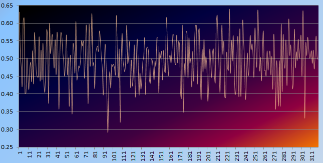
Figure 1: Example of time series with no periodicity and no trend (up or down)
I computed the median, 25- and 75-percentiles for the first few records, see Figure 2. For instance, the median time of occurrence of the first record (after the first measurement) is after 2 years, if your time unit is a year. The next bigger record is expected 8 years after the first measurement, and the next bigger one 21 years after the first measurement (see Figure 2.) Even if you look at the 25-percentile, it really takes a lot of years to beat the previous 4 or 5 records in a row. In short, it is nearly impossible to observe increasing records four years in a row, unless there is a trend that forces the observed values to become larger over time.
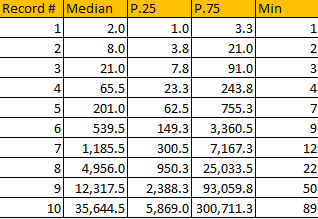
Figure 2: Time of arrivals of successive records (in years if you time unit is a year)
This study of arrival times for these records should allow you to detect even very tiny trends, either up or down, better than traditional models of change point detection hopefully. However it does not say anything about whether the increase is barely perceptible or rather large.
Note that the values of these records is a subject of much interest in statistics, known as extreme value theory. This theory has been criticized for failure to predict the amount of damage in modern cataclysms, resulting in big losses for insurance companies. Part of the problem is that these models are based on hundreds of years worth of data (for instance to predict the biggest flood that can occur in 500 years) but over such long periods of time, the dynamics of the processes at play have shifted. Note that here, I focus on the arrival times or occurrences of these records, not on their intensity or value, contrarily to traditional extreme value theory.
Finally, arrival times for these records do not depend on the mean or variance of the underlying distribution. Figure 2 provides some good approximations, but more tests and simulations are needed to confirm my findings. Are these median arrival times the same regardless of the underlying distribution (temperature, stock market prices, and so on) just like the central limit theorem provides a same limiting distribution regardless of the original, underlying distribution? The theoretical statistician should be able to answer this question. I didn’t find many articles on the subject in the literature, though this one is interesting. In the next section, I try to answer this question. The answer is positive.
2. Theoretical Distribution of Records over Time
This is an interesting combinatorial problem, and it bears some resemblance to the Analyticbridge Theorem. Let R(n) be the value of the n-th record (n = 1, 2,…) and T(n) its arrival time.
For instance, if the data points (observed values) are X(0) = 1.35, X(1) = 1.49, X(2) = 1.43, X(3) = 1.78, X(4) = 1.63, X(5) = 1.71, X(6) = 1.45, X(7) = 1.93, X(8) = 1.84, then the records (highlighted in bold) are R(1) = 1.49, R(2) = 1.78, R(3) = 1.93, and the arrival times for these records are T(1) = 1, T(2) = 3, and T(3) = 7.
To compute the probability P(T(n) = k) for n > 0 and k = n, n+1, n+2, etc., let’s define T(n, m) as the arrival time of the n-th record if we only observe the first m+1 observations X(0), X(1) … X(m). Then P(Tn) = k) is the limit of P(T(n,m) = k) as m tends to infinity, assuming the limit exists. If the underlying distribution of the values X(0), X(1), etc. is continuous, then, due to the symmetry of the problem, computing P(T(n,m) = k) can be done as follows:
- Create a table of all (m+1)! (factorial m+1) permutations of (0, 1, … , m).
- Compute N(n, m, k), the number of permutations of (0, 1, …, m) where the n-th record occurs at position k in the permutation (with 0 < k <= m). For instance, if m = 2, we have 6 permutations (0, 1, 2), (0, 2, 1), (1, 0, 2), (1, 2, 0), (2, 0, 1) and (2, 1, 0). The first record occurs at position k = 1 only for the following three permutations: (0, 1, 2), (0, 2, 1), and (1, 2, 0). Thus, N(1, 2, 1) = 3. Note that the first element in the permutation is assigned position 0, the second one is assigned position 1, and so on. The last one has position m.
- Then P(T(n,m) = k) = N(n, m, k) / (m+1)!
As a result, the distribution of arrival times, for the records, is universal: it does not depend on the underlying distribution of the identically and independently distributed observations X(0), X(1), X(2) etc.
It is easy (with or without using my above combinatorial framework) to find that the probability to observe a record (any record) at position k is 1 / (k+1) assuming again that the first position is position 0 (not 1). Also, it is easy to prove that P(T(n) = n) = 1 / (n+1)!. Now, T(1) = k if and only if X(k) is a record among X(0), …, X(k) and X(0) is the largest value among X(0), …, X(k-1). Thus:
P(T(1) = k) = 1 / { (k+1) * k }
This result is confirmed by my simulations. For the general case, recurrence formulas can be derived.
3. Useful Results
None of the arrival times T(n) for the records has a finite expectation. Figure 3 displays the first few values for the probability that the n-th record occurs at position T(n) = k, the first element in the data set being assigned to position 0. The distribution of of these arrival times does not depend on the underlying distribution of the observations.
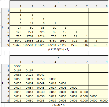 Figure 3: P(T(n) = k) at the bottom, (k+1)! P(T(n) = k) at the top
These probabilities were computed using a small script that generates all (k+1)! permutations of (0, 1, …, k) and checks, among these permutations, those having a record at position k: for each of these permutations, we computed the total number of,records. If N(n, k) denotes the number of such permutations having n records, then P(T(n) = k) = N(n,k) / (k+1)!.
Despite the fact that the above table is tiny, it required hundreds of millions of computations for its production.
Top DSC Resources
- Article: Difference between Machine Learning, Data Science, AI, Deep Learnin…
- Article: What is Data Science? 24 Fundamental Articles Answering This Question
- Article: Hitchhiker’s Guide to Data Science, Machine Learning, R, Python
- Tutorial: Data Science Cheat Sheet
- Tutorial: How to Become a Data Scientist – On Your Own
- Categories: Data Science – Machine Learning – AI – IoT – Deep Learning
- Tools: Hadoop – DataViZ – Python – R – SQL – Excel
- Techniques: Clustering – Regression – SVM – Neural Nets – Ensembles – Decision Trees
- Links: Cheat Sheets – Books – Events – Webinars – Tutorials – Training – News – Jobs
- Links: Announcements – Salary Surveys – Data Sets – Certification – RSS Feeds – About Us
- Newsletter: Sign-up – Past Editions – Members-Only Section – Content Search – For Bloggers
- DSC on: Ning – Twitter – LinkedIn – Facebook – GooglePlus
Follow us on Twitter: @DataScienceCtrl | @AnalyticBridge