State-of-the-Art Machine Learning Automation with HDT

The technique presented here blends non-standard, robust versions of decision trees and regression. It has been successfully used in black-box ML implementations.

In this article, we discuss a general machine learning technique to make predictions or score transactional data, applicable to very big, streaming data. This hybrid technique combines different algorithms to boost accuracy, outperforming each algorithm taken separately, yet it is simple enough to be reliably automated It is illustrated in the context of predicting the performance of articles published in media outlets or blogs, and has been used by the author to build an AI (artificial intelligence) system to detect articles worth curating, as well as to automatically schedule tweets and other postings in social networks.for maximum impact, with a goal of eventually fully automating digital publishing. This application is broad enough that the methodology can be applied to most NLP (natural language processing) contexts with large amounts of unstructured data. The results obtained in our particular case study are also very interesting.

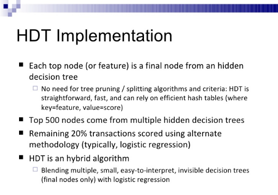
Figure 1: HDT 1.0. Here we describe HDT 2.0.

The algorithmic framework described here applies to any data set, text or not, with quantitative, non-quantitative (gender, race) or a mix of variables. It consists of several components; we discuss in details those that are new and original, The other, non original components are briefly mentioned, with references provided for further reading. No deep technical expertise and no mathematical knowledge is required to understand the concepts and methodology described here. The methodology, though state-of-the-art, is simple enough that it can even be implemented in Excel, for small data sets (one million observations.).

1. The Problem

Rather than first presenting a general, abstract framework and then showing how it applies to a specific problem (case study), we decided to proceed the other way around, as we believe that it will help the reader understand better our methodology. We then generalize to any kind of data set.

In its simplest form, our particular problem consists of analyzing historical data about articles and blog posts, to identify features (also called metrics or variables) that are good predictors of blog popularity when combined together, to build a system that can predict the popularity of an article before it gets published. The goal is to select the right mix of relevant articles to publish, to increase web traffic, and thus advertising dollars, for a niche digital publisher.

As in any similar problem, the historical data is called training set, and it is split into test data and control data for cross-validation purposes to avoid over-fitting. The features are selected to maximize some measure of predictive power, as described here. All of this is (so far) standard practice; the reader not familiar with this can Google the keywords introduced in this paragraph. In our particular case, we use our domain expertise to identify great features. These features are pretty generic and apply to numerous NLP contexts, so you can re-use them for your own data sets.

Feature Selection and Best Practices

One caveat is that some metrics are very sensitive to distortion. In our case, the response (that is, what we are trying to predict, also called dependent variable by statisticians) is the traffic volume. It can be measured in page views, unique page views, or number of users who read the article. Page views can easily be manipulated and the number is inflated by web robots, especially for articles that have little traffic. So instead, we chose “unique page views”, a more robust metric available through Google Analytics. Also, older articles have accumulated more page views over time, so we need to correct for this effect. Correcting for time is explained in this article. Here we used a very simple approach instead: focusing on articles from the most recent, big channel instead (the time window is about two years), and taking the logarithm of unique page views (denoted as pv in the source code in the last section).

Taking the logarithm not only smooths out the effect of time and web robots, but also it makes perfect sense as the page view distribution is highly skewed — well modeled using a Zipf distribution — with a few incredibly popular (viral) articles and a large number of articles with average traffic: it is a bit like the income distribution.

As for selecting the features, we have two kinds of metrics that we can choose as predictors:

1. Metrics based on the article title, easy to compute:

Keywords found in the title
Article category (blog, event, forum question)
Channel
Creation date
Title contains numbers?
Title is a question?
Title contains special characters?
Length of title

2. Metrics based on the article body, more difficult to compute:

Size of article
Does it contain pictures?
Keywords found in body
Author (and author popularity)
First few words

Despite focusing only on a subset of features associated with the article title, we were able to get very interesting, actionable insights; we only used title keywords, and whether the posting is a blog, or not. You have to keep in mind that the methodology used here takes into account all potential key-value combinations, where a key is a subset of features, and value, the respective values: for instance key = (keyword_1, keyword_2, article category) and value = (“Python”, “tutorial”, “Blog”). So it is important to appropriately bin the variables when turning them into features, to prevent the number of key-value pairs from exploding. Another mechanism described further down in this article is also used to keep the key-value database, stored as an hash table or associate array, manageable. Finally, it can easily be implemented in a distributed environment (Hadoop.)

Due to the analogy with decision trees, a key-value is also called a node, and plays the same role as a node in a decision tree.

2. Methodology and Solution

As we have seen in the previous section, the problem consists of predicting pv, the logarithm of unique page views for an article (over some time period), as a function of keywords found in the title, and whether the article in question is a blog or not.

In order to do so, we created lists of all one-token and two-token keywords found in all the titles, as well as blog status, after cleaning the titles and eliminating some stop word such as “that”, “and” or “the”, that don’t have impacts on the predictions. We were also careful about not eliminating all keywords made up of one or two letters: the one-letter keyword “R”, corresponding to the programming language R, has a high predictive power.

For each element in our lists, we recorded the frequency and traffic popularity. More precisely, for each key-value pair, we recorder the number of articles (titles, actually) that are associated with it, as well as the average, minimum and maximum pv across these articles.

Example

For instance, the element or key-value (keyword_1 = “R”, keyword_2 = “Python”, article = “Blog”) is associated with 6 articles, and has the following statistics: avg pv = 8.52, min pv = 7.41, and max pv = 10.45.

Since the average pv across all articles is equal to 6.83, this specific key-value pair (also called node) generates exp(8.52 – 6.83) = 5.42 times more traffic than an average article. It is thus a great node. Even the worst article, among the 6 articles belonging to this node, with a pv of 7.41, outperforms the average article across all nodes. So not only this is a great node, but also a stable one. Some nodes have a far larger volatility, for instance when one of the keywords has different meanings, such as the word “training”, in “training deep learning” (training set) versus “deep learning training” (courses.)

Hidden decision trees (HDT) revisited

Note that here, the nodes are overlapping, allowing considerable flexibility. In particular, nodes with two keywords are sub-nodes of nodes with one keyword. A previous version of this technique, described here, did not consider overlapping nodes. Also, with highly granular features, the number of nodes explodes exponentially. A solution to this problem consists of

shuffling the observations
working with nodes built on no more than 4 or 5 features
proper binning
visiting the observations sequentially (after the shuffle) and every one million observations, deleting nodes that contain only one observation

The general idea behind this technique is to group articles into buckets that are large enough to provide predictions that are sound, without explicitly building decision trees. Not only the nodes are simple and easy to interpret, but unstable nodes are easy to detect and discard. There is no splitting/pruning involved as with classical decision trees, making this methodology simple and robust, and thus fit for artificial intelligence (automated processing.)

General framework

Whether you are dealing with predicting the popularity of an article, or the risk for a client to default on a loan, the basic methodology is identical. It involves training sets, cross-validation, feature selection, binning, and populating hash tables of key-value pairs (referred to here as the nodes).

When you process a new observation, you check which node(s) it belongs to. If the best node it belongs to is stable and not too small, you use it to predict the future performance or value of your observation, or to score the transaction if you are dealing with transactional data such as credit card transactions. In our example, if the performance metric (the average pv in the node in question) is significantly above the global average, and other constraints are met (the node is not too small, and the minimum pv in the node in question not too low to guarantee stability), then we classify the observation as good, just like the node it belongs to. In our case, the observation is a potential article.

Also, you need to update your training set and the node table (including automatically discovered new nodes) every six months or so.

Parameters must be calibrated to guarantee that

error rate (classifying a good observation as bad or the other way around) is small enough; it is measured using a confusion matrix
the system is robust: we have a reasonable number of stable nodes that are big enough; it is great if less than 3,000 stable, not too small nodes cover 80% of the observations (by stable, we mean nodes with low variance) with an average of at least 10 observations per node
the binning and feature selection mechanism offer real predictive power: the average response (our pv) measured in a node classified as good, is much above the general average, and the other way around for nodes classified as bad; in addition, the response shows little volatility within each node (in our case, pv is relatively stable across all observations within a same usable node)
we have enough usable nodes (that is, after excluding the small ones) to cover at least 50% of all observations, and if possible up to 95% of all observations (100% would be ideal but never exists in practice)

We discuss the parameters of our technique, and how to fine-tune them, in the next section. Fine-tuning can be automated or made more robust by testing (say) 2,000 sets of parameters and identify regions of stability that meet our criteria (in terms of error rate and so on) in the parameter space.

A big question is what to do with observations not belonging to any usable node: they can not be classified. In our example it does not matter if 30% of the observations can not be classified, but in many applications, it does matter. One way to address this issue is to use super-nodes: in our case, a node for all posts that are blogs, and another one for all posts that are not blogs (these two nodes cover 100% of observations, both past and future.) The problem is that usually, these super-nodes don’t have much predictive power. A better solution consists of using two algorithms: the one described here based on usable nodes (let’s call it algorithm A) and another one called algorithm B, that classifies all observations. Observations that can’t be classified or scored with algorithm A are classified/scored with algorithm B. You can read the details about how to blend the results of two algorithms, in one of my patents. In practice, we have used Jackknife regression for algorithm B, a technique easy to implement, easy to understand, leading to simple interpretations, and very robust. These feature are important for systems that are designed to run automatically.

The resulting hybrid algorithm is called Hidden Decision Trees – hidden because you don’t even realize that you have created a bunch of mini decision trees: it was all implicit. The version described here is version 2, with new features to prevent the node table from exploding, and allowing nodes to overlap, making it more suitable for data sets with a larger number of variables.

3. Case Study: Results

Our application about predicting page views for an article has been explained in detail in the previous sections. So here we focus on the results obtained.

Output from the algorithm

If you run the script listed in the next section, besides producing the table of key-value pairs (the nodes) as a text file for further automated processing, it displays summary statistics that look like the following:

Average pv: 6.81
Number of articles marked as good: 865 (real number is 1079)
Number of articles marked as bad: 1752 (real number is 1538)
Avg pv: articles marked as good: 8.23
Avg pv: articles marked as bad: 6.13
Number of false positive: 50 (bad marked as good)
Number of false negative: 264 (good marked as bad)
Number of articles: 2617
Error Rate: 0.12
Number of feature values: 16712 (marked as good: 3409)
Aggregation factor: 1.62

The number of “feature values” is the total number of key-value pairs found, including the small unstable ones, regardless as to whether they are classified as good or bad. Any article with a pv above the arbitrary value pv_threshold = 7.1 (see source code) is considered as good. This corresponds to articles having about 1.3 times more traffic than average, since we use a log scale and the average pv is 6.81. The traffic for articles classified as good by the algorithm (pv = 8.23) is about 4.2 times above the traffic that an average article receives.

Two important metrics are:

Aggregation factor: it is an indicator of the average size of a node. The minimum is 1, corresponding to nodes that only have one observation. A value above 5 is highly desirable, but here, because we are dealing with a small data set and with niche articles, even a small value is OK.
The error rate is the number of articles wrongly classified. Here we care much more about bad articles classified as good.

Also note that we correctly identify the vast majority of good articles, but this is because we work with small nodes. Finally an article is marked as good if it triggers at least one node marked as good (that is, satisfying the criterion defined in the next sub-section.)

Parameters

Besides pv_threshold, the algorithm uses 12 parameters to identify a usable, stable node classified as good. These parameters are illustrated in the following piece of code (see source code):

if ( (($n > 3)&&($n < 8)&&($min > 6.9)&&($avg > 7.6)) ||
(($n >= 8)&&($n < 16)&&($min > 6.7)&&($avg > 7.4)) ||
(($n >= 16)&&($n < 200)&&($min > 6.1)&&($avg > 7.2)) ) {

Here, n represents the number of observations in a node, while, avg and min are the average and minimum pv for the node in question. We tested many combinations of values for these parameters. Increasing the required size (denoted as n)of a usable node will do the following:

decrease the number of good articles correctly identified as good
increase the error rate
increase the stability of the system
decrease the predictive power
increase the aggregation factor (see previous sub-section)

Improving the methodology

Here we share some caveats and possible improvements to our technique.

You need to use a table of one-token keywords that look like two tokens, for increased efficiency, and consider these keywords as being one-token. For instance “San Francisco” is a one-token keyword, despite its appearance. Such tables are easy to build as you always see the two parts together.

Also, we looked at nodes containing (keyword_1, keyword_2) where the two keywords are adjacent. If you allow the two keywords not to be adjacent, the number of key-value pairs (the nodes) increases significantly, but you don’t get much additional predictive power in return: there is even a risk of over-fitting.

Another improvement consists of having/favoring nodes containing observations spread over a long time period, to avoid any kind of concentration (which could otherwise result in over-fitting.)

Finally, in our case, we can not exclusively focus on articles with great potential. It is important to have many, less popular articles as well: they constitute the long tail. Without these articles, we face problems such as excessive content concentration, which have negative impacts in the long term. The obvious negative impact is that we might miss nascent topics, and thus getting stuck into an non-adaptive mix of articles at some point, thus slowing growth.

Interesting findings

Titles with the following features work well:

contains a number (10, 15 and so on) as we have many popular articles such as “10 great deep learning articles”.
contains the current year (2017)
is a question (how to)
not a blog, but a book category
a blog

Titles containing the following keywords work well:

everyone (as in “10 regression techniques everyone should know”)
libraries
infographic
explained
algorithms
languages
amazing
must read
r python
job interview questions
should know (as in “10 regression techniques everyone should know”)
nosql databases
versus
decision trees
logistic regression
correlations
tutorials
code
free

Recommended reading

You might also like my related articles about a data scientists sharing his secrets, and turning unstructured data into structured data. To read my best data science and machine learning articles, click here.

4. Source Code

The source code is easy to read and has deliberately made longer than needed to provide enough details, avoid complicated iterations, and facilitate maintenance and translation into Python or R. The output file hdt-out2.txt stores the key-value pairs (or nodes) that are usable, corresponding to popular articles. Here is the input data set: HDT-data3.txt.

The code has been written in Perl, R and Python. Perl and Python run faster than R. Click on the relevant link below to access the source code, available as a text file. The code was originally written in Perl, and translated to Python and R by Naveenkumar Ramaraju who is currently pursuing a master’s in Data Science at Indiana University

Python version
Perl version
R version
Improved R version

For those learning Python or R, this is a great opportunity. HDT (a light version) has been implemented in Excel too: click here to get the spreadsheet (you will have to scroll down to the middle of section 3, just above the images.)

Note regarding the R implementation

Required library: hash (R doesn’t have inbuilt hash or dictionary without imports.) You can use any one of below script files.

Standard version is the literal translation of the Perl code with same variable names to the maximum extent possible.
Improved version uses functions, more data frames and more R-like approach to reduce code running time (~30 % faster) and less lines of code. Variable names would vary from Perl. Output file would have comma(,) as delimiter between IDs.

Instructions to run: Place the R file and HDT-data3.txt (input file) in root folder of R environment. Execute the ‘.R’ file in R studio or using command line script:

> Rscript HDT_improved.R

R is known to be slow in text parsing. We can optimize further if all inputs are within double quotes or no quotes at all by using data frames.

Julia version

This was added later by Andre Bieler. The comments below are from him.

For what its worth, I did a quick translation from Python to Julia (v0.5) and attached a link to the file below, feel free to share it. I stayed as close as possible to the Python version, so it is not necessarily the most “Julian” code. A few remarks about benchmarking since I see this briefly mentioned in the text:

This code is absolutely not tuned for performance since everything is done in global scope. (In Julia it would be good practice to put everything in small functions)
Generally for run times of only a few 0.1 s Python will be faster due to the compilation times of Julia.

Julia really starts paying off for longer execution times. Click here to get the Julia code.

For related articles from the same author, click here or visit www.VincentGranville.com. Follow me on on LinkedIn.

DSC Resources