
Some original and very interesting material is presented here, with possible applications in Fintech. No need for a PhD in math to understand this article: I tried to make the presentation as simple as possible, focusing on high-level results rather than technicalities. Yet, professional statisticians and mathematicians, even academic researchers, will find some deep and fascinating results worth further exploring. Source code and Excel spreadsheets are provided for replication purposes.
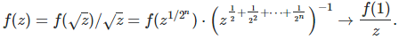
Let’s start with
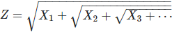
Here the X(k)’s (k = 1, 2 and so on) are random variable identically and independently distributed. This is the first time ever that nested square roots involving random variables are investigated. We are trying to find the distribution of Z. Of course, Z has the same distribution as SQRT(X + Z) where X has the same distribution of X(1), X(2) and so on. In short, we are trying to solve the functional equation
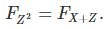
The notation F stands for the distribution function as usual.
1. Using a Simple Discrete Distribution for X
What seems at first glance to be the most simple case is as follows. Use a Bernouilli distribution of parameter p = 1/2 for X. The resulting support domain for Z is then [1, (1+SQRT(5)) / 2]. The upper bound is attained when all X(k)’s are equal to 1. The lower bound is attained when all but one of the X(k)’s are equal to 0. If all X(k)’s are zero, then Z = 0, but this happens with probability zero, so 0 is a singularity and not part of the support domain for Z.
Despite the simplicity of the model, Z has a highly chaotic, complex distribution, and its support domain is full of gaps, some pretty large. So we will not study this model. If you are interested in it, read this document or a recent PhD thesis on the subject, entitled Continued Radicals and Cantor Sets, available here.
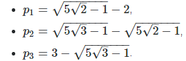
Another simple model that comes to mind, and indeed much more tractable, consists of using a 3-parameter discrete distribution for X, defined as follows: P(X = 0) = p(1), P(X = 1) = p(2), P(X = 2) = p(3) = 1 – p(1) – p(2). Now the support domain for Z is [1, 2] and the gaps are eliminated if the three parameters p(1), p(2) and p(3) are strictly positive. Yet the distribution for Z is still very wild unless the three parameters are carefully chosen. For instance if these parameters are as follows:
You would think that this set of parameters leads to a uniform distribution on [1, 2], for Z. This is because these three values correspond to the equilibrium distribution in the numeration system based on nested radicals: see my article Number Representation Systems Explained in One Picture, published here (see column labeled “nested square root”, with row labeled “digits distribution”.) However this is not the case. The reason is that the X(k)’s (each representing a random digit in the nested radical numeration system) are slightly auto-correlated at equilibrium, unlike the digits in standard numeration systems. But here the X(k)’s are not auto-correlated in my model, and thus Z does not have a uniform distribution.
You may ask, what about using p(1) = p(2) = p(3) = 1/3 instead? Now this leads to a very chaotic system. It’s like using random digits in the standard binary numeration system, if you choose for the probability of a digit to be 1 or 0, a value different from 1/2. It actually leads to a very similar distribution (for Z) as the one depicted in my article A Strange Family of Statistical Distributions, available here.
2. Towards a Better Model
It is easy, using the 3-parameter discrete distribution for X discussed in section 1, to prove the following:
Here f represents the density attached to Z. Because of these equations, Z‘s distribution can not be uniform, quadratic or any polynomial. Of course this assumes that Z has a density. I believe it does not, though it has a distribution F. In order words, F is nowhere differentiable. More on this soon, but for now let’s pretend that Z has a density. A nice set of parameters in that case, would be p(1) = 1/2, p(2) = 1 / (1 + SQRT(5)), and p(3) = (3 – SQRT(5)) / 4. The reason for this is explained here, see section “Third Update.” We would then have:
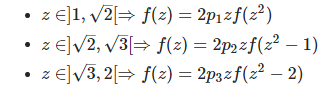
Case 1:
Here z is in ]1, SQRT(2) [, then
Case 2:
Here z is in ]SQRT(2), SQRT(3) [. Let’s introduce the following notation:

and so on. Then we have:
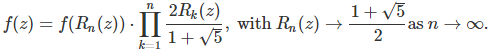
Note that the above product converges as n tends to infinity. More about this here.
Case 3:
Here z is in ]SQRT(3), 2[. This case is left as an exercise.
Note that f may not exist, much less be continuous, so the limit in case 1 does not make sense. However case 1 suggests that F(z) — which exists and is obtained by integrating f(z) — could be a logarithm function. It turns out that indeed, this provides an excellent approximation.
2.1. Approximate Solution
With the discrete distribution for X mentioned at the beginning of section 2, that is p(1) = 1/2, p(2) = 1 / (1 + SQRT(5)), and p(3) = (3 – SQRT(5)) / 4, we have the following excellent approximation for the distribution of Z:
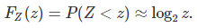
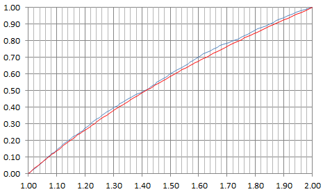
See chart below, with the logarithm approximation in red, and the actual distribution of Z in blue. The support domain for Z is the interval [1, 2].
2.2. The Fractal, Brownian-like Error Term
Here we discuss in more details the error term
The curve below represents E(z). Before reading any further, can you identify some patterns?
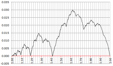
Note that the error is maximum at z = (1 + SQRT(5)) / 2. Notable local minima for E(z) include (among infinitely many others) z = 1, 2^(1/4), SQRT(2), SQRT(3) and z = 2. Also, the curve seems to be differentiable nowhere, indeed it has some of the patterns of a Brownian motion. In particular, one can see a fractal behavior, with the successive double-bumps (followed and preceded by a big dip all the way down to E(z) = 0) repeating themselves over time but being amplified as z increases. The maximum attained at each double-bump seems to be exactly 2 times the maximum reached at the previous double-bump. Each double-bump looks like a Brownian Bridge, though somewhat smoother, probably with a Hurst exponent higher than 1/2.
Furthermore, it seems that the median is SQRT(2), though I haven’t checked. Now if you switch the values of p(1) and p(3), then it looks like the median becomes SQRT(3). And if p(1) = p(2) = p(3) = 1/3 (a very chaotic case), it looks like the median becomes (1 + SQRT(5)) / 2.
3. Finding X and Z Using Characteristic Functions
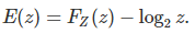
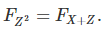
Here we consider a more general approach, assuming a continuous distribution for X. A characteristic function uniquely identifies a distribution: there is a one-to-one mapping between the two concepts, involving a Fourier transform. If ξ is the characteristic function (CF) of Z^2, ψ is the CF of Z, ϕ is the CF of X(k), and if ϕ = ξ / ψ, then the distribution of the nested square root of the X(k)’s is also the distribution of Z. This is a simple application of the convolution theorem for Y = X + Z, with Y having the distribution of Z^2, and X, Z being independent.
We want to find simple distributions for X and Z, such that the functional equation listed at the beginning of this article, namely
is satisfied. This guarantees that the distribution of Z is actually that of the infinite nested radicals. The idea is to first find some Z (that is, ξ and ψ), compute the ratio of the two CF’s. If this ratio is the CF of some distribution X, then we solved the problem in a backward way, by specifying the distribution of Z first, and then finding that of X. Note that Z can not have a log-normal distribution, because Z can not be lower than 1. A potential candidate for Z‘s distribution is log-log-normal, that is log log Z is normal.
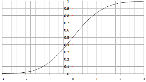
3.1. Test with Log-normal Distribution for X
As a first attempt at trying to find an elegant solution using empirical means, I decided to pick up a log-normal distribution for X as it has desirable features: the square root of a log-normal distribution is also log-normal, but unfortunately the sum of log-normal distributions is not log-normal; you can’t have it all. The following chart is based on X being log-normal, more specifically with log X being Normal(0, 1). It looks like log log Z is almost normal, yet as in the example in section 2, it is only an approximation. A very good one, but not an exact solution. Below is the chart for the empirical distribution of log log Z (after rescaling to produce mean = 0 and variance = 1), based on 10,000 deviates, each involving 400 X(k)’s. It looks almost perfectly normal! Normal deviates were produced using the Box Muller transform.
I haven’t studied the approximation error like I did in section 2 for a discrete X. I leave it to you as an exercise. You can find how good the approximation is by looking at my spreadsheet, available here: compare columns I and K. The source code (in Perl) to produce both Z and Normal(0, 1) deviates, is displayed below, and also available as a text file, here.
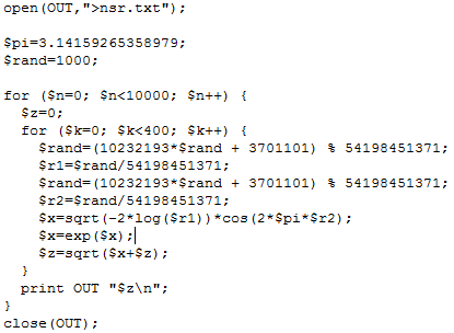
Note that in the code, I replaced the built-in Rand function by one of my own: this is because the Perl Rand function is pretty terrible, able to generate only 32,768 distinct values; the issue is described here. If you write your code in Python, you won’t have this problem.
3.2. Playing with the Characteristic Functions
Here I try do do the opposite of the approach in section 3.1: first specifying the distribution of Z, then finding that of X using the characteristic functions relationship mentioned at the beginning of section 3, that is ϕ = ξ / ψ. Very few cases lead to simple integration, but f(z) = 2z / 3 with z in [1, 2], for the density attached to Z, is one of them. Using WolframAlpha to compute integrals, it leads to
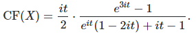
Here again, CF denotes the characteristic function. However, it turns out that CF(X) is NOT a characteristic function. In other words, it is impossible to find a distribution for X that would result in the desired distribution for Z. The problem is similar if instead you consider rescaling / averaging infinitely many X(k)’s, and denote the result as Z. You can’t pre-specify the distribution of Z, and hope that there is an X that works: Z must always be Gaussian due to the central limit theorem (except in few cases, see here). In short, the possibilities for the distribution of Z for infinite nested radicals, are also limited. The distributions that do work are called attractors in chaos theory, and the distribution whose density is f(z) = 2z / 3 is not one of them. It would be interesting to characterize the set of all attractor distributions for infinite nested radicals.
Also, as discussed in section 2, Z might not have a density. In this case, the classical theory of Fourier transforms may not apply, and characteristic functions could be meaningless in that context. Some new mathematical tools must be designed to handle such cases.
3.3. Generalization to Continued Fractions and Nested Cubic Roots
Consider

This generalizes the nested radicals problem. Again, the X(k)’s are independently and identically distributed. Nested radicals correspond to α = 1/2. Nested cubic roots correspond to α = 1/3, while continued fractions correspond to α = -1. The relationship ϕ = ξ / ψ between the characteristic functions is unchanged, but this time ξ is the characteristic function of Z^(1/α).
4. Exercises
While we have been working so far with nested radicals of random variables, the exercises below focus on deterministic sequences.
[1] Let us consider the following nested square root:
Prove the following:
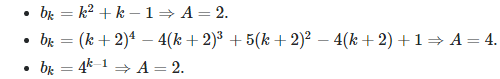
The first two cases involve an algorithm with

The first case corresponds to α = 1, the second case to α = 2. See solution here.
[2] Let
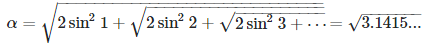
Prove that α is not the square root of π. Solution: see here.
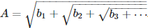
[3] Taylor series for special nested square roots. Let

Prove that 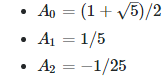
Can you compute the next three coefficients? Solution: see here. Note the limit of f(x), as x tends to 0+, is not equal to 1 despite the appearances. It is equal to SQRT(2). Also, f(x) does not have a Taylor series expansion around x = 0.