
This simple introduction to matrix theory offers a refreshing perspective on the subject. Using a basic concept that leads to a simple formula for the power of a matrix, we see how it can solve time series, Markov chains, linear regression, data reduction, principal components analysis (PCA) and other machine learning problems. These problems are usually solved with more advanced matrix calculus, including eigenvalues, diagonalization, generalized inverse matrices, and other types of matrix normalization. Our approach is more intuitive and thus appealing to professionals who do not have a strong mathematical background, or who have forgotten what they learned in math textbooks. It will also appeal to physicists and engineers. Finally, it leads to simple algorithms, for instance for matrix inversion. The classical statistician or data scientist will find our approach somewhat intriguing.
1. Power of a Matrix
For simplicity, we illustrate the methodology for a 2 x 2 matrix denoted as A. The generalization is straightforward. We provide a simple formula for the n-th power of A, where n is a positive integer. We then extend the formula to n = -1 (the most useful case) and to non-integer values of n.
Using the notation
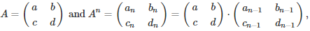
we obtain
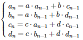
Using elementary substitutions, this leads to the following system:
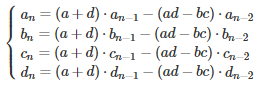
We are dealing with identical linear homogeneous recurrence relations. Only the initial conditions corresponding to n = 0 and n = 1, are different for these four equations. The solution to such equations is obtained as follows (see here for details.) First, solve the quadratic equation
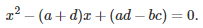
The two solutions r(1), r(2) are
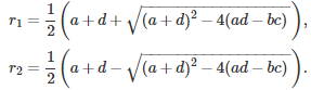
If the quantity under the square root is negative, then the roots are complex numbers. The final solution depends on whether the roots are distinct or not:
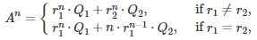
with
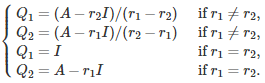
Here the symbol I represents the 2 x 2 identity matrix. The last four relationships were obtained by applying the above formula for A^n, with n = 0 and n = 1. It is easy to prove (by recursion on n) that this is the correct solution.
If none of the roots is zero, then the formula is still valid for n = -1, and thus it can be used to compute the inverse of A.
2. Examples, Generalization, and Matrix Inversion
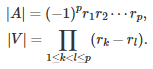
For a p x p matrix, the methodology generalizes as follows. The quadratic polynomial becomes a polynomial of degree p, known as the characteristic polynomial. If its roots are distinct, we have
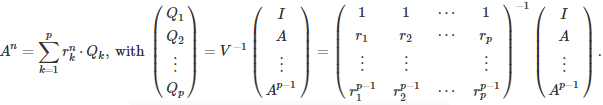
The matrix V is a Vandermonde matrix, so there is an explicit formula to compute its inverse, see here and here. A fast algorithm for the computation of its inverse is available here. The determinants of A and V are respectively equal to
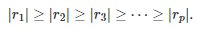
Note that the roots can be real or complex numbers, simple or multiple, or equal to zero. Usually the roots are ordered by decreasing modulus, that is
That way, a good approximation for A^n is obtained by using the first three or four roots if n > 0, and the last three or four roots if n < 0. In the context of linear regression (where the core of the problem consists of inverting a matrix, that is, using n = -1 in our general formula) this approximation is equivalent to performing a principal component analysis (PCA) as well as PCA-induced data reduction.
If some roots have a multiplicity higher than one, the formulas must be adjusted. The solution can be found by looking at how to solve an homogeneous linear recurrence equation, see theorem 4 in this document.
2.1. Example with a non-invertible matrix
Even if A is non-invertible, some useful quantities can still be computed when n = -1, not unlike using a pseudo-inverse matrix in the general linear model in regression analysis. Let’s look at this example, using our own methodology:
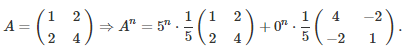
The rightmost matrix attached to the second root 0 is of particular interest, and plays the role of a pseudo-inverse matrix for A. If that second root was very close to zero rather than exactly zero, then the term involving the rightmost matrix would largely dominate in the value of A^n, when n = -1. At the limit, some ratios involving the (non-existent!) inverse of A still make sense. For instance:
- The sum of the elements of the inverse of A, divided by its trace, is (4 – 2 – 2 + 1) / (4 + 1) = 1 / 5.
- The arithmetic mean divided by the geometric mean of its elements, is 1 / 2.
2.2. Fast computations
If n is large, one way to efficiently compute A^n is as follows. Let’s say that n = 100. Do the following computations:
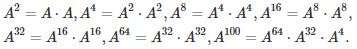
This can be useful to quickly get an approximation of the largest root of the characteristic polynomial, by eliminating all but the first root in the formula for A^n, and using n = 100. Once the first root has been found, it is easy to also get an approximation for the second one, and then for the third one.
If instead, you are interested in approximating the smallest roots, you can proceed the other way around, by using the formula for A^n, with n = -100 this time.
3. Application to Machine Learning Problems
We have discussed principal component analysis, data reduction, and pseudo-inverse matrices in section 2. Here we focus on applications to time series, Markov chains, and linear regression.
3.1. Markov chains
A Markov chain is a particular type of time series or stochastic process. At iteration or time n, a system is in a particular state s with probability P(s | n). The probability to move from state s at time n, to state t at time n + 1 is called a transition probability, and does not depend on n, but only on s and t. The Markov chain is governed by its initial conditions (at n = 0) and the transition probability matrix denoted as A. The size of the transition matrix is p x p, where p is the number of potential states that the system can evolve to. As n tends to infinity A^n and the whole system reaches an equilibrium distribution. This is because
- The characteristic polynomial attached to A has a root equal to 1.
- The absolute value of any root is less than or equal to 1.
3.2. AR processes
Auto-regressive (AR) processes represent another basic type of time series. Unlike Markov chains, the number of potential states is infinite and forms a continuum. Yet the time is still discrete. Time-continuous AR processes such as Gaussian processes, are not included in this discussion. An AR(p) process is defined as follows:
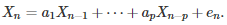
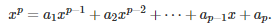
Its characteristic polynomial is
Here { e(n) } is a white noise process (typically uncorrelated Gaussian variables with same variance) and we can assume that all expectations are zero. We are dealing here with a non-homogeneous linear (stochastic) recurrence relation. The most interesting case is when all the roots of the characteristic polynomial have absolute value less than 1. Processes satisfying this condition are called stationary. In that case, the auto-correlations are decaying exponentially fast.
The lag-k covariances satisfy the relation

with

Thus the auto-correlations can be explicitly computed, and are also related to the characteristic polynomial. This fact can be used for model fitting, as the auto-correlation structure uniquely characterizes the (stationary) time series. Note that if the white noise is Gaussian, then the X(n)’s are also Gaussian.
The results about the auto-correlation structure can be found in this document, pages 98 and 106, originally posted here. See also this this document (pages 112 and 113) originally posted here, or the whole book (especially chapter 6) available here. See also section 4 (Appendix.)
3.3. Linear regression
Linear regression problems can be solved using the OLS (ordinary least squares) method, see here. The framework involves a response y, a data set X consisting of p features or variables and m observations, and p regression coefficients (to be determined) stored in a vector b. In matrix notation, the problem consists of finding b that minimizes the distance ||y – Xb|| between y and Xb. The solution is
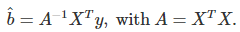
The techniques discussed in this article can be used to compute the inverse of A, either exactly using all the roots of its characteristic polynomial, or approximately using the last few roots with the lowest moduli, as if performing a principal component analysis. If A is not invertible, the methodology described in section 2.1. can be useful: it amounts to working with a pseudo inverse of A. Note that A is a p x p matrix as in section 2.
Questions regarding confidence intervals (for instance, for the coefficients) can be addressed using the model-free re-sampling techniques discussed in my article confidence intervals without pain.
4. Appendix
Here we connect the dots between the auto-regressive time series described in section 3.2., and the material in section 2. For the AR(p) process in section 3.2., we have
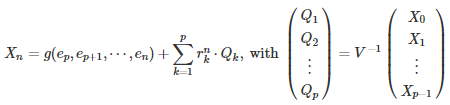
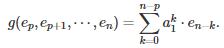
where V is the same matrix as in section 2, the r(k)’s are the roots of the characteristic polynomial (assumed distinct here), and g is a linear function of e(p), e(p+1), …, e(n). For instance, if p = 1, we have
 This formula allows you to compute Var[X(n)] and Cov[X(n), X(n–k)], conditionally to X(0), …, X(p-1). The limit, when n tends to infinity, allows you to compute the unconditional variance and auto-correlations attached to the process, in the stationary case. For instance, if p = 1, we have
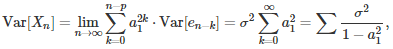
where sigma square is the variance of the white noise, and |a(1)| < 1 because we assumed stationarity.
For the general case (any p) the formula, if n is larger than or equal to p, is
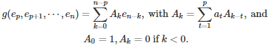
The initial conditions for the coefficients A(k) correspond to k = 0, -1, -2, …, -(p -1), as listed above. The recurrence relation for A(k), besides the initial conditions, is identical to the previous one and thus can be solved with the same p x p matrix V and the same roots. If two time series models, say an ARMA and an AR models, have the same variance and covariances, they are actually identical.
To not miss this type of content in the future, subscribe to our newsletter. For related articles from the same author, click here or visit www.VincentGranville.com. Follow me on on LinkedIn, or visit my old web page here.