
Convolution is a concept well known to machine learning and signal processing professionals. In this article, we explain in simple English how a moving average is actually a discrete convolution, and we use this fact to build weighted moving averages with natural weights that at the limit, have a Gaussian behavior guaranteed by the Central Limit Theorem. Moving averages are nothing more than blurring filters for signal processing experts, with a Gaussian-like kernel in the case discussed here. Inverting a moving average to recover the original signal consists in applying the inverse filter, known as a sharpening or enhancing filter. The inverse filter is used for instance in image analysis, to remove noise or deblur an image, while the original filter (the moving average) does the opposite. This is discussed here for one dimensional discrete signals, known as time series. Generalizations are also discussed. An interesting application in number theory, related to the famous unsolved Riemann conjecture, is also discussed.
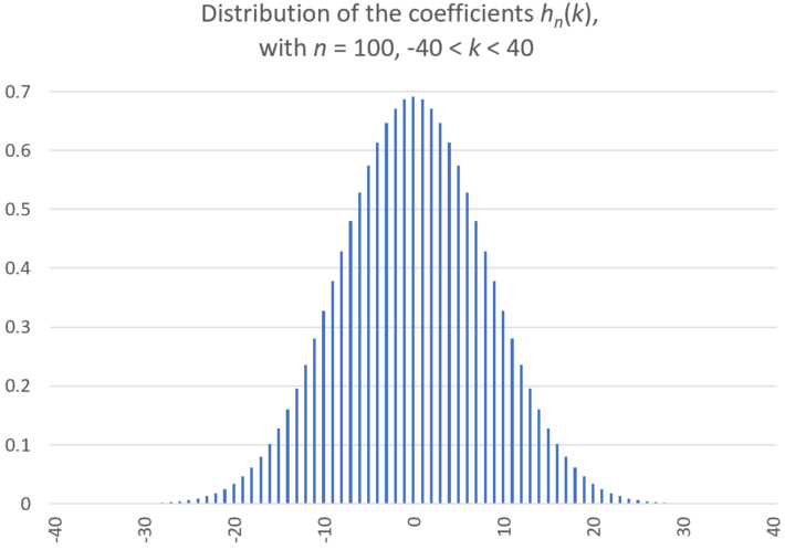
Figure 1: Bell-shaped distribution for re-scaled coefficients (the weights) discussed in section 1.1
1. Weighted moving averages as convolutions
Given a discrete time series with observations X(0), X(1), X(2) and so on, a weighted moving average can be defined by
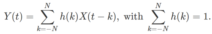
Here Y(t) is the smoothed signal and h is a discrete density function (thus summing to one) though negative values of h(k) are sometimes used, for instance in Spencer’s 15-point moving average used by actuaries, see here. We assume that t can take on negative integer values. Also, unless otherwise specified, we assume the weights to be symmetrical, that is, h(k) = h(-k). The parameter N can be infinite, but typically, the values h(k) are fast decaying the further away you are from k = 0.
The notation used by mathematicians to represent this transformation is as follows: Y = T(X) = h * X where * is the convolution operator. This notation is convenient because it easily allows us to define the iterated moving average as a self-composition of the operator T, acting on the time series X : Start with Y0 = X, Y1 = Y, and let Yn+1 = T(Yn) = h * Yn. Likewise, we can define hn (with h1 = h) as h * h * … * h, that is, an n-fold self-convolution of h. Of course, Yn = hn * X so that we have
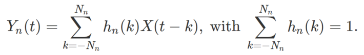
Note that the sum goes from –Nn to Nn this time, as each additional iteration increases the number of terms in the sum, so Nn+1 > Nn, with N1 = N. This becomes clear in the following illustration.
1.1 Example
The most basic case corresponds to N = 1, with h(-1) = h(0) = h(1) = 1/3. In this case, Nn = n, and the average value of hn(k) is equal to 1 / (2Nn +1). We have the following table:
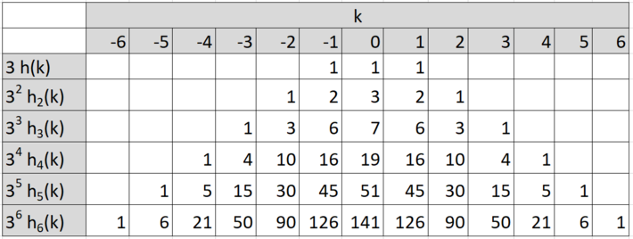
The above table shows how the weights are automatically determined, without guess work, rule of thumb, or fine-tuning required. Note that the sum of the elements in the n-th row is always equal to 3^n (3 at power n). This is very similar to the binomial coefficients table, and hn(k) are known as the trinomial coefficients, see here. The difference is that for binomial coefficients, the sum of the elements in the n-th row is always equal to 2^n, and the n-th row only has n + 1 entries, versus 2n + 1 in our table. The values hn(k) corresponding to n = 100 are displayed in Figure 1, at the top of this article. They have been scaled by a factor equal to the square root of Nn, since otherwise they all tend to zero as n tends to infinity.
1.2 Link to the Central Limit Theorem
The methodology developed here can be used to prove the central limit theorem in the most classic way. Indeed, the classic proof uses iterated self-convolutions, and the fact that the Fourier transform of convolutions is the product of the individual Fourier transform of each convolution. The Fourier transform is called characteristic function in probability theory. Interestingly, this leads to Gaussian approximations for partial sums of coefficients such as those in the n-th row, in the above table, when n is large and after proper rescaling. This is already well known for binomial coefficients (see here), and it easily extends to the coefficients introduced here, as well as to many other types of mathematical coefficients. See also Figure 1.
2. Inverting a moving average, and generalizations
Inverting a moving average consists in retrieving the original time series or signal. It consists in applying the inverse filter to the observed data, to un-smooth it. It is usually not possible to do it, though the true answer is somewhat more nuanced. It is certainly easier to do when N is small, though usually N is not known, and the weights are also unknown. However if the observed data is the result of applying the simple convolution described in section 1.2 with N = 1, you only need to know the values of X(t) at two different times t0 and t1 to retrieve the original signal. This is easiest if you know X(t) at t0 = 0 and at t1 = 1: in this case, there is a simple inversion formula:

If you know X(0), X(1), and Y(t) for all t‘s, you can iteratively retrieve X(2), X(3), and so on with the above recurrence formula. If you don’t know X(0), X(1) but instead you know the variance and other higher moments of X(t), assuming X(t) is stationary, then you may test various X(0), X(1) until you find a pair matching these moments when reconstructing the full sequence X(t) using the above recurrence formula. The solution may not be unique. Other parameters you know about X(t) may be useful too for the reconstruction: the period (if any), the slope of a linear trend (if any), and so on.
2.1 Generalizations
The moving averages discussed here rely on the classic arithmetic mean as the fundamental convolution operator, corresponding to N = 1. It is possible to use other means such as the harmonic or geometric means, and even more general as those defined in this article. It can be generalized to two or higher dimensions, and to a time-continuous signal. For prediction or extrapolation, see this article. For interpolation, that is to estimate X(t) when t is not an integer, see this article.
3. Application and source code
We applied the above methodology with n = 60 to the following time series, with 60 < t < 240 being an integer:
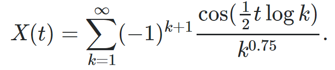
Figure 2 shows Yn(t) with n = 60 (the red curve), after shifting and rescaling (multiplying) it by a factor of order sqrt(n). In this case, X(2t) represents the real part of the Dirichlet Eta function η defined in the complex plane. If you replace the cosine by a sine in the definition of X(t), you get similar results for the imaginary part of η. What is spectacular here is that Yn(t) is very well approximated by a cosine function, see bottom of figure 2. The implication is that thanks to the self-convolution used here, we can approximate the real and imaginary parts of η by a simple auto-regressive model. This in turn may have implications to help solve the famous Riemann Hypothesis (RH) which essentially consists in locating the values of t such that X(2t) = 0 simultaneously for the real and imaginary part of η. RH states that there is no such t in our particular case, where a parameter 0.75 is used in the definition of X(t). It is conjectured to also be true if you replace 0.75 by any value strictly between 0.5 and 1. See more here and here.
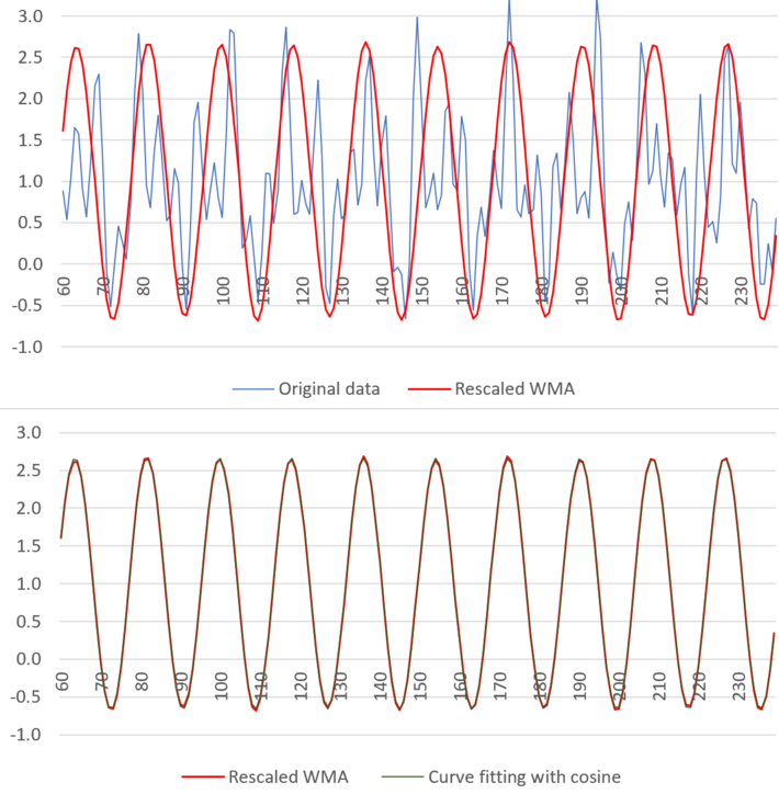
Figure 2: weighted moving average (WMA) with n = 60 (top), model fitting with cosine function (bottom)
Note that X(t), the blue curve, is non-periodic, while the red curve is almost perfectly periodic. If you use arbitrary moving averages instead of the one based on a convolution hn * X, you won’t get a perfect fit in the bottom part of figure 2, certainly not a perfect fit with a simple cosine function. 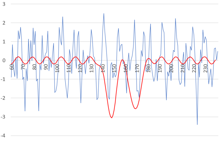
Figure 3: same as top part of figure 2, but using a different X(t) for the blue curve
Also, the perfect fit can not be achieved if you replace the logarithm in the definition of X(t), by a much faster growing function. This is illustrated in figure 3, where the logarithm in X(t) was replaced by a square root.
The source code can be downloaded here (convol2b.pl.txt). Since it is dealing with convolutions, it can be further optimized using Fast Fourier Transforms (FFT), see here. Finally, it would be interesting to treat this case assuming the time t is continuous, using continuous rather than discrete convolutions.
About the author: Vincent Granville is a data science pioneer, mathematician, book author (Wiley), patent owner, former post-doc at Cambridge University, former VC-funded executive, with 20+ years of corporate experience including CNET, NBC, Visa, Wells Fargo, Microsoft, eBay. Vincent also founded and co-founded a few start-ups, including one with a successful exit (Data Science Central acquired by Tech Target). He is also the founder and investor in Paris Restaurant in Anacortes, WA. You can access Vincent’s articles and books, here.