
This is the second part of my article Spectacular Visualization: The Eye of the Riemann Zeta Function, focusing on the most infamous unsolved mathematical conjecture, one that has a $1 million dollar price attached to it. I used the word deep not in the sense of deep neural networks, but because the implications of these visualizations have deep consequences on how to solve this conjecture, opening a new path of attack and featuring non-standard generalizations leading to new perspectives and new approaches so solve RH (as the conjecture is called in mathematical circles).
This work is mostly based on data science, and the results presented here are experimental in nature and still need to be proved formally. The main visualization featuring 6 scatterplots is published here for the first time: it shows the orbits of 3 Riemann-like functions, their eyes, and their surprising ring-shaped error distribution when only the first few hundred terms are used in the series defining these functions. It deviates from classical pure-math approaches in the sense that what I do looks more like stochastic dynamical systems, attractors, wavelets, and should appeal to data analysts, engineers and physicists.
The problem is so popular that there are YouTube videos about it, some having gathered several million of views. One of them is also featured here. My own scatterplots show the behavior of a new class of Riemann-like functions, as well as interesting slices of the orbit that are rarely (if ever) displayed in the literature, revealing peculiar features that could help in solving RH.
1. Orbits of Riemann-like Functions
The main picture in this article consists of the 6 plots below. Click on the picture to zoom in.
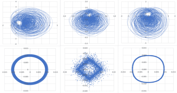
Figure 1: Orbit (top) and residual error (bottom) for cosine (left), triangular (middle) and square wave (right)
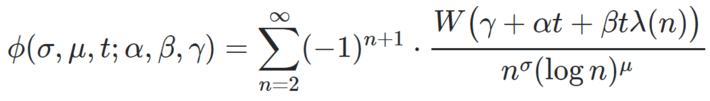
I explain later in this section what they represent. But first, I need to introduce some material. Let
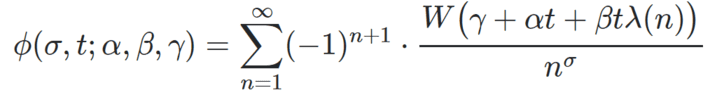
be a function of t, with 0.5 < σ < 1 fixed, and α, β, γ three real parameters. This generalizes the function ϕ introduced in my previous article. This time, λ(n) = n and α = 0, β = 1. Also, we are dealing with two sister functions of t, namely ϕ1(σ, t) = ϕ(σ, t; α, β, γ) with γ = 0, and the shifted ϕ2(σ, t) = ϕ(σ, t; α, β, γ) with γ = -π/2. They represent respectively the real and imaginary part of some function defined on the complex plane. The Riemann Hypothesis (RH), corresponding to W(x) = cos x, states that there is no zero of the Riemann zeta function ζ(s), with s = σ + it a complex number, if 0.5 < σ < 1. Here i represents the imaginary unit whose square is -1. In layman’s term, it means that we can not have ϕ1(σ, t) = ϕ2(σ, t) = 0 if 0.5 < σ < 1. You win $1 million if you prove it, see here.
The novelty in my method is the introduction of a periodic wave function W in the definition of ϕ, thus generalizing RH in a way different from what other mathematicians did, that is, without using complicated L-functions. This offers more hopes to solve Riemann’s conjecture (RH), by first trying to prove it for the easiest W, and understand what those W‘s having an RH attached to them (as opposed to those that do not) have in common.
Figure 1 (upper part) displays the spectacular orbits for three different waves (cosine, triangular and alternating-quadratic) in the test case σ = 0.75 and 0 < t < 600, with the hole around the origin (I call it the eye) being the hallmark of RH behavior: that is, no root for that particular value of σ, regardless of t, because of the hole. Though not displayed here, in the case σ = 0.5, the hole is entirely gone and corresponds to the critical line (the name given by mathematicians) where all the zeroes are found.
The orbit consists, for a fixed σ, of the points (X(t),Y(t)) with X(t) = ϕ1(σ, t) and Y(t) = ϕ2(σ, t). The bottom three plots represent the error between the true value (X(t),Y(t)) and its approximation based on using only the first 200 terms in the series that defines ϕ. The error distribution is very surprising; I was expecting the points to be radially but randomly distributed around the origin; instead, they are located on a ring. Note that for t > 600 (and for the triangular wave, for t > 80) you need to use more than 200 terms for the pattern to remain strong.
In Figure 1, the left part of the plot corresponds to the cosine wave (that is, classical RH), the middle part corresponds to the triangular wave, and the right part corresponds to the alternating quadratic wave. Interestingly, when σ = 1/2 the orbit does not have a hole anymore as predicted, yet the error points are still distributed on a similar ring.
The wave W is a continuous periodic function of period 2π, with one minimum equal to −1 and one maximum equal to +1 in the interval [0,2π], and the area below the X-axis equal to the area above the X-axis. It must have some symmetry. The waves used here are defined as follows:
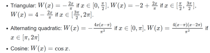
For the cosine wave, the Taylor series for ϕ is discussed here, while the representation as an infinite product is discussed here.
2. Other interesting visualizations
The orbit for the standard RH case has been published countless time for σ = 0.5. In that case, there is no eye as the orbit crosses the origin infinitely many times. Some videos about the orbit trajectory have been posted on You Tube and viewed millions of times. Below is one of them.
Other popular visualizations include the time series for ϕ1(σ, t) and ϕ2(σ, t) when σ = 0.5. Below (Figure 2) is a version of mine, for σ = 0.75 and 0 < t < 600. Not only it displays the time series for the cosine wave (standard RH case) but also for the triangular wave, for the first time ever. The blue curve corresponds to ϕ1(σ, t), the orange one to ϕ2(σ, t).
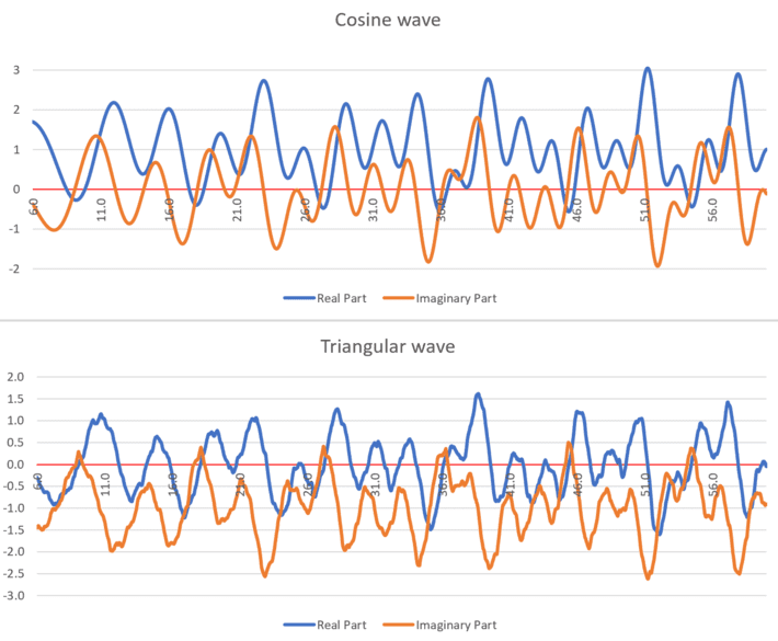
Figure 2: Time series for ϕ1(σ, t) and ϕ2(σ, t) when σ = 0.75
It is interesting to notes that the peaks and valley floors of the triangular and cosine wave frameworks seem to be correlated, occurring at similar times. What’s more, for the cosine wave, when a zero of the blue curve is close to a zero of the orange curve (that is then these curves cross the X-axis at a similar time), the zero of the orange curve occurs first. This seems to be true too for the triangular wave, at least when t < 600.
3. Generalization and source code
The Perl source code is available here. Note that convergence is very slow, as discussed in my previous article. A table of the first 100,000 zeros of ζ(s) can be found here. More general results are available here. In short, if 0.5 < σ < 1, the hole around the origin (pictured in Figure 1) is also present in the following case. Let’s define
together with ϕ1(σ, t) = 1 + ϕ(σ, μ, t; α, β, γ) with γ = 0, and ϕ2(σ, t) = ϕ(σ, μ, t; α, β, γ) with γ = -π/2. Then we still have a hole around the origin. That hole persists even if σ = 0.5, unless μ = 0. Here μ, σ are fixed but arbitrary, λ(n) = log n, and α = 0, β = 1; only t varies. It has been tested only for W(x) = cos x, and when 0 < t < 200.
Exercise 1
Show (numerically) that the cross-correlation between ϕ1(σ, t) and ϕ2(σ, t) is apparently zero, for the cosine wave W(x) = cos x. However, if you shift the orange curve in Figure 2, replacing ϕ2(σ, t) by ϕ2(σ, t + τ), the correlation may no longer be zero. Find τ (numerically) that maximizes the cross-correlation in question.
Exercise 2
Prove that if ζ(s) = 0, with s = σ + it and 0 < σ < 1 then for all real θ, we have
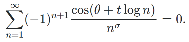
See answer here.
Exercise 3
Prove that the centroid of the orbits pictured in Figure 1, is always (W(0), W(-π/2)). This is true for the cosine, triangular and alternate square waves. Hint: The integral of W(x) between x = 0 and x = 2π (the period) is always zero. The coordinates of the centroid are
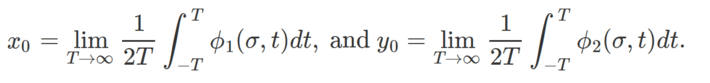
Since ϕ1, ϕ2 are defined as infinite sums, swap the integral and sum operators, then proceed to the computation. The integral vanishes for all the terms in both series, except for the first one where it is equal to W(0) and W(-π/2), respectively for ϕ1 and ϕ2.
About the author: Vincent Granville is a data science pioneer, mathematician, book author (Wiley), patent owner, former post-doc at Cambridge University, former VC-funded executive, with 20+ years of corporate experience including CNET, NBC, Visa, Wells Fargo, Microsoft, eBay. Vincent also founded and co-founded a few start-ups, including one with a successful exit (Data Science Central acquired by Tech Target). You can access Vincent’s articles and books, here.