
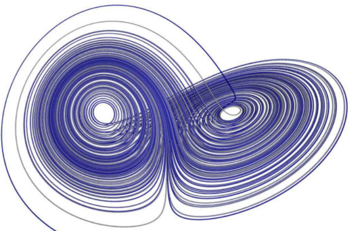
Dynamical system used in weather prediction (see here)
We are dealing here with random variables recursively defined by Xn+1 = g(Xn), with X1 being the initial condition. The examples discussed here are simple, discrete and one-dimensional: the purpose is to illustrate the concepts so that it can be understood and useful to a large audience, not just to mathematicians. I wrote many articles about dynamical systems, see for example here. The originality in this article is that the systems discussed are now random, as X1 is a random variable. Applications include the design of non-periodic pseudorandom number generators, and cryptography. Also, such systems, especially more complex ones such as fully stochastic dynamical systems, are routinely used in financial modeling of commodity prices.
We focus on mappings g on the fixed interval [0, 1]. That is, the support domain of Xn is [0, 1], and g is a many-to-one mapping onto [0,1]. The most trivial example, known as the dyadic or Bernoulli map, is when g(x) = 2x – INT(2x) = { 2x } where the curly brackets represent the fractional part function (see here). This is sometimes denoted as g(x) = 2x mod 1. The most well-known and possibly oldest example is the logistic map (see here) with g(x) = 4x(1 – x).
We start with a simple exercise that requires very little mathematical knowledge, but a good amount of out-of-the-box thinking. The solution is provided. The discussion is about a specific, original problem, referred to as the inverse problem, and introduced in section 2. The reasons for being interested in the inverse problem are also discussed. Finally, I provide an Excel spreadsheet with all my simulations, for replication purposes. Before discussing the inverse problem, we discuss the standard problem in section 1.
1. The standard problem
One of the main problems in dynamical systems is to find if the distribution of Xn converges, and find the limit, called invariant measure, invariant distribution, fixed-point distribution, or attractor. The attractor, depending on g, is typically the same regardless of the initial condition X1, except for some special initial conditions causing problems (this set of bad initial conditions has Lebesgue measure zero, and we ignore it here). As an example, with the Bernoulli map g(x) = { 2x }, all rational numbers (and many other numbers) are bad initial conditions. They are however far outnumbered by good initial conditions. It is typically very difficult to determine if a specific initial condition is a good one. Proving that Ï/4 is a good initial condition for the Bernoulli map would be a major accomplishment, making you instantly famous in the mathematical community, and proving that the digits of Ï in base 2, behave exactly like independently and identically distributed Bernoulli random variables. Good initial conditions for the Bernoulli map are called normal numbers in base 2.
It is also assumed that the dynamical system is ergodic: all systems investigated here are ergodic; I won’t elaborate on this concept, but the curious, math-savvy reader can check the meaning on Wikipedia. Finding the attractor is a difficult problem, and it usually requires solving a stochastic integral equation. Except in rare occasions (discussed here and in my book, here), no exact solution is known, and one needs to use numerical methods to find an approximation. This is illustrated in section 1.1., with the attractor found (approximately) using simulations in Excel. In section 2., we focus on the much easier inverse problem, which is the main topic of this article.
1.1. Standard problem: example
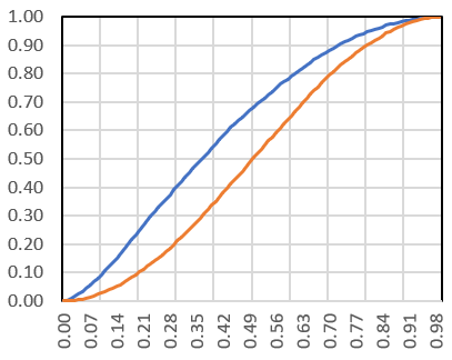
Let’s start with X1 defined as follows: X1 = U / (1 – U)^α, where U is a uniform deviate on [0, 1], α = 0.25, and ^ denotes the power operator (2^3 = 8). We use g(x) = { 4x(1 – x) }, where { } denotes the fractional part function. Essentially, this is the logistic map. I produced 10,000 deviates for X1, and then applied the mapping g iteratively to each of these deviates, up to Xn with n = 53. The scatterplot below represents the empirical percentile distribution function (PDF), respectively for X3 in blue, and X53 in orange. These PDF’s, for X2, X3, and so on, slowly converge to a limit, corresponding to the attractor. The orange S-curve (n = 53) is extremely close to the limiting PDF, and additional iterations (that is, increasing n) barely provide any change. So we found the limit (approximately) using simulations. Note that the cumulative distribution function (CDF) is the inverse of the PDF. All this was done with Excel alone.
2. The inverse problem
The inverse problem consists of finding g, assuming the attractor distribution (the orange curve in the above figure) is known. Typically, there are many possible solutions. One of the possible reasons for solving the inverse problem is to get a sequence of random variables X1, X2, and so on, that exhibits little or no auto-correlations. For instance, the lag-1 auto-correlation (between Xn and Xn+1) for the Bernoulli map, is 1/2, which is way too high depending on the applications you have in mind. It is important in cryptography applications to remove these auto-correlations. The solution proposed here also satisfies the following property: X2 = g(X1), X3 = g(X2), X4 = g(X3) and so on, all have the same pre-specified attractor distribution, regardless of the (non-singular) distribution of X1.
2.1. Exercise
Before diving into a solution, if you have time, I ask you to solve the following simple inverse problem.
Find a mapping g such that if Xn+1 = g(Xn), the attractor distribution is uniform on [0, 1]. Can you find one yielding very low auto-correlations between the successive Xn‘s? Hint: g may not be continuous.
2.2. A general solution to the inverse problem
A potential solution to the problem in section 2.1 is g(x) = { bx } where b is an integer larger than 1. This is because the uniform distribution on [0, 1] is the attractor for this map. The case b = 2 corresponds to the Bernoulli map discussed earlier. Regardless of b, INT(bXn) represents the n-th digit of X1, in base b. The lag-1 autocorrelation between Xn and Xn+1, is then equal to 1 / b. Thus, the higher b, the better. Note that if you use Excel for simulations, avoid even integer values for b, as Excel has an internal glitch that will make your simulations meaningless after n = 45 iterations or so.
Now, a general solution offered here, for any pre-specified attractor and any non-singular distribution for X1, is based on a result proved here. If g is the solution in question, then all Xn (with n > 1) have the same distribution as the pre-specified attractor. I provide an Excel spreadsheet showing how it works for a specific example.
First, let’s assume that g* is a solution when the attractor is the uniform distribution on [0, 1]. For instance g*(x) = { bx } as discussed earlier. Let F be the CDF of the target attractor, and assume its support domain is [0, 1]. Then a solution g is given by
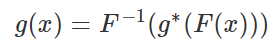
For instance, if F(x) = x^2, with x in [0, 1], then g(x) = SQRT( { bx^2 } ) works, assuming b is an integer larger than 1. The scatterplot below shows the empirical CDF of X2 (blue dots, based on 10,000 deviates) versus the CDF of the target attractor with distribution F (red curve): they are almost indistinguishable. I used b = 3, and for X1, I used the same distribution as in section 1.1. The detailed computations are available in my spreadsheet, here (13 MB download).
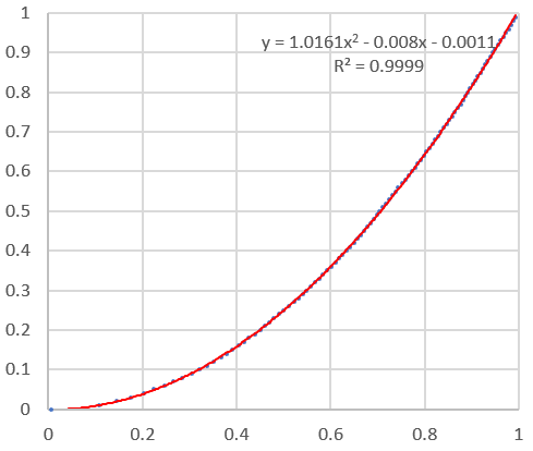
The summary statistics and the above plot are found in columns BD to BH, in my spreadsheet.
To receive a weekly digest of our new articles, subscribe to our newsletter, here.
About the author: Vincent Granville is a data science pioneer, mathematician, book author (Wiley), patent owner, former post-doc at Cambridge University, former VC-funded executive, with 20+ years of corporate experience including CNET, NBC, Visa, Wells Fargo, Microsoft, eBay. Vincent is also self-publisher at DataShaping.com, and founded and co-founded a few start-ups, including one with a successful exit (Data Science Central acquired by Tech Target). You can access Vincent’s articles and books, here.