
Update: Part 2 of this article is now available, here.
In this article, original stochastic processes are introduced. They may constitute one of the simplest examples and definitions of point processes. A limiting case is the standard Poisson process – the mother of all point processes – used in so many spatial statistics applications. We first start with the one-dimensional case, before moving to 2-D. Little probability theory knowledge is required to understand the content. In particular, we avoid discussing measure theory, Palm distributions, and other hard-to-understand concepts that would deter many readers. Nevertheless, we dive pretty deep into the details, using simple English rather than arcane abstractions, to show the potential. A spreadsheet with simulations is provided, and model-free statistical inference techniques are discussed, including model-fitting and test for radial distribution. It is shown that two realizations of very different processes can look almost identical to the naked eye, while they actually have fundamental differences that can only be detected with machine learning techniques. Cluster processes are also presented in a very intuitive way. Various probability distributions, including logistic, Poisson-binomial and Erlang, are attached to these processes, for instance to model the distribution and/or number of points in some area, or distances to nearest neighbors.
1. The one-dimensional case
I stumbled upon the processes in question while trying to generalize mathematical series (in particular for the Riemann-zeta function) to make them random, replacing the values of the index in the summation formula by locations close to the deterministic equally-spaced values (integers k = 0, 1, 2, 3 and so on), to study the behavior. I ended up with a point process defined as follow, on the real line (the X-axis):
1.1. Definitions
Let Fs be a continuous cumulative distribution function (CDF) symmetrical and centered at 0, belonging to a parametric family of parameter s, where s is the scaling factor. In short, s is an increasing function of the variance. If s = 0, the variance must be zero, and if s is infinite, the variance must be infinite. Due to symmetry, the expectation is zero.
Let (Xk) be an infinite sequence of independent random variables, where k takes on any positive or negative integer value. By definition, the distribution of Xk is Fs(x – k) and is thus centered at k. So, P(Xk < x) = Fs(x – k). If s = 0, Xk = k. Our point process consists of all the points Xk, and this is how this stochastic point process is defined.
Now let B = [a, b], with a < b, be any interval on the real line. We define the following basic quantities:
- N(B) is a random variable counting the number of points, among the Xk‘s, that are in B.
- pk = P(N(B) = k) is the probability that there are exactly k points in B
Typical distributions for Fs are uniform, Gaussian, Cauchy, Laplace, or logistic, centered at zero. By construction, the process is stationary. Also, two points corresponding to two different indices h, k can not share the same location: that is, with probability one, Xh can not be equal to Xk unless h = k. These trivial facts, combined with knowing the distribution of N(B) for any B, uniquely characterizes the type of point process we are dealing with. For instance, if N(B) had a Poisson distribution, then we would be dealing with a stationary Poisson point process on the real line, with intensity λ = 1.
1.2. Fundamental results
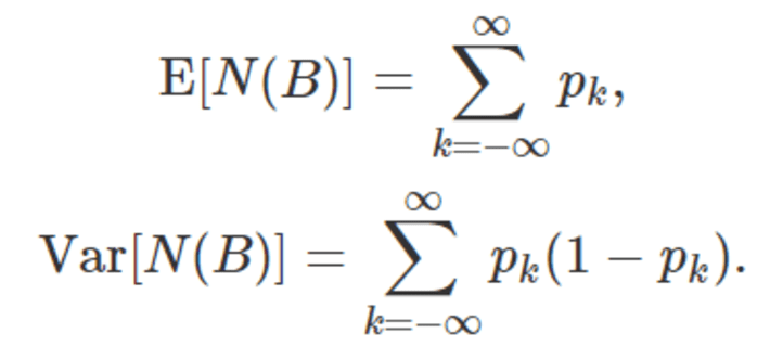
Here E denotes the expectation, and Var denotes the variance. Fundamental results include:
- E[N(B)] = b – a if b – a is an integer, just like for a stationary Poisson process of intensity λ = 1
- N(B) never has a Poisson distribution, thus the process is never Poisson
- N(B) has a Poisson-binomial distribution (see definition here and illustration here) of parameters p0, p1, p2 and so on, regardless of Fs
- When s tends to infinity, the process so defined tends to a stationary Poisson process of intensity λ = 1 on the real line, regardless of Fs
The first result is easy to prove, you can try to prove it yourself first, as an exercise. The answer is found here, see Theorem A. Note that for N(B), we have a Poisson-binomial distribution with an infinite number of parameters; the standard Poisson-binomial distribution only has a finite number of parameters. When I first analyzed this type of processes, I made some mistakes. These were corrected in a peer-reviewed discussion, see here.
Two fundamental quantities are the expectation and variance of N(B):
1.3. Distributions of interest and discussion
In one dimension, unlike a Poisson point process, the points are more evenly distributed than if they were purely randomly distributed, with potential applications to generating quasi-random or low-discrepancy sequences, typically used in numerical integration. The opposite is true in two dimensions, as we shall see in section 2.
Also the characteristic function CF, the moment generating function MGF and the probability generating function PGF of N(B) are known, since N(B) has a discrete Poisson-binomial distribution: see here. The granularity of the process is one, since the indices (the k‘s) are integers and the distance between two successive integers is always one. This results in the density (actually called intensity and denoted as λ) of points in any interval being a constant equal to one. However, if you choose a finer granularity, that is, a lattice with evenly spaced k‘s closer to each other by a factor (say) 5, the intensity is multiplied by the factor in question (5, in this case). In short, if k is replaced by k/λ , then the intensity of the process is λ.
Distributions of interest include:
- Interarrival times (also called distances, or waiting times in queuing theory) between two successive points (also called events in queuing theory): in the case of a Poisson process, it would have an exponential distribution, and the distribution of the waiting time between n occurrences of the event would have an Erlang distribution, see here. In two dimensions, arrival times are replaced by distances to the nearest neighbor, and the distribution is well known and easy to establish, see here. It can easily be generalized to k-nearest neighbors, see the first page, first paragraph of this article. But in our case, we are not dealing with Poisson processes, and the distribution must be approximated using simulations.
- The point distribution (the way the Xk‘s are distributed): it would be uniform on any compact set in any dimension if the process was a stationary Poisson process, a fact easy to establish. But here again, we are not dealing with Poisson processes, and the distribution must be approximated using simulations.
Some formulas are available in closed form for particular cases, especially for the moments of the random variable N(B). This is the case if Fs is a uniform or Laplace distribution. We will mention just one of these formulas, for the expectation of N(B) if Fs is a uniform distribution on [1-s, 1+s]. The details for this laborious but trivial computation can be found here.
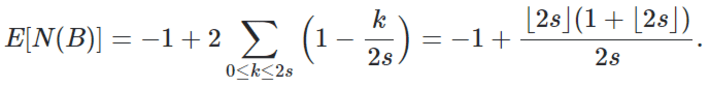
Here the brackets represent the integer part function. This formula is correct if B = [-s, s]. When s is an integer or half an integer, it is exactly equal to 2s, the length of the interval B. This is in agreement with the first property mentioned at the beginning of section 1.2. And when s tends to infinity, it is also asymptotically equivalent to 2s. This is in agreement with the fact that as s tends to infinity, the process tends to a stationary Poisson process of intensity λ = 1.
2. The two-dimensional case
In two dimensions, the index k becomes a two dimensional index (h, k), and the point Xk becomes a vector (Xh, Yk). It is tempting to use, for the distribution of (Xh, Yk), the joint density Fs(x, y) = Fs(x)Fs(y), thus assuming independence between X and Y, and the same scaling factor for both X and Y.
In the simulations below, I used only one index k, with Xk replaced by a bivariate vector (Xk, Yk), with Xk and Yk independent. Thus the two coordinates of each point are paired, as in paired time series (an unpaired version is discussed in part 2 of this article). This does not work well if s is small, as the points obviously get highly concentrated near the main diagonal in that case, as seen in figures 1 (a) and 1 (d) below. The issue is easily fixed by applying a 45 degree clockwise rotation so that the main diagonal becomes the X-axis, and the correlation between the two coordinates drops from almost 1 to almost 0. Then you need to rescale (say) the X variable, by multiplying all the Xh‘s by a same factor, so that at the end, both variances, for the Xh‘s and the Yk‘s, are identical or at least very close to each other. This is similar to applying a Mahalanobis transformation to the original 2-D process. The resulting process is called the rescaled process.
Note that in the figures below, the intensity chosen for the process is 100, not 1. But in the end, it does not matter as far as understanding the principles, or applying the methodology, is concerned. It’s purely a cosmetic change.
2.1. Simulations
I simulated a realization of a point process, for four different types of processes, each time with 1,000 points. The index k ranges from -5 to +5 with increments equal to 1/100. Figure 1 shows the result for small values of s, and Figure 2 for large values of s. Each figure features 6 plots:
- Plot (a): Raw 2-D process, with Fs being a logistic distribution (see here) of parameter s.
- Plot (b): Rescaled version of (a), as discussed above.
- Plot (c): Stationary point Poisson process of similar intensity.
- Plot (d): Raw 2-D process, with Fs being a uniform distribution on [-s, s].
- Plot (e): Rescaled version of (c), as discussed above.
- Plot (f): Process with radial intensity (to be discussed in Part 2 of this article)
See the plots below.
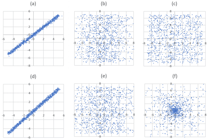
Figure 1: small s
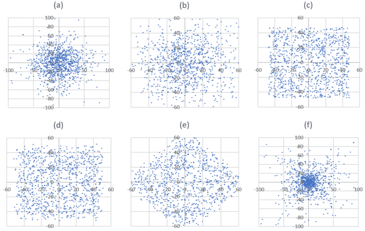
Figure 2: large s
Note that the full process, with k covering all the positive and negative integers, would cover the entire plane. Here we only see a finite window as we are using a finite number of k‘s in the simulations. In part 2 of this article, I show how it looks like when using an infinite number of points, in the case of a cluster process.
2.2. Interpretation
The number of points in any circle of radius r centered at the origin, divided by the area of the circle in question, is denoted as N(r). For the Poisson process (plot (c)), the number N(r) is almost constant: not statistically different from being constant, if you exclude small values of r for which N(r) is too small to get any meaningful conclusion, and values of r too large with the circle overshooting the limit of the square window used in the simulation.
For the radial process, N(r) is very large for small r, but decreases exponentially fast as r is increasing. It is easy to test that this process is not Poisson, as we shall see in the second part of this article. Surprisingly, despite the appearances, the processes based on Fs (I will call them Poisson-binomial processes) are somewhat closer to the radial than the Poisson process when s is small, if you look at N(r). You don’t see it because:
- The radial process has a few points (not many) spreading far away outside the origin and even well beyond the window, while the Poisson-binomial process lacks this feature, which to the naked eye, artificially magnifies the difference between the two.
- Most importantly, there is something special, more difficult to pinpoint, between figure 1 (b) and 1 (e) which are truly very similar, and figure 1 (c) which is radically different from 1 (b) or 1 (e) despite the appearances: 1 (b) and 1(e) are somewhat closer to 1 (f) than to 1 (c). Can you guess why? Look at these plots for 30 seconds, three feet away from your screen before reading the next sentence. The explanation is this: points in figures 1 (b) and 1 (e) are far more concentrated around the Y-axis than points in figure 1 (c) which are randomly distributed. And this is more difficult to see to the naked eye because of peculiarities of our brain circuity. But a statistical test will detect it very easily.
In short, the radial process exhibits a radial point concentration (by design), while the Poisson-binomial process built as described above (by rescaling the X axis), exhibits a similar concentration but this time around the Y axis, when s is small. There is also a border effect: using a finite number of k‘s has a bigger impact when s is small, in terms of distorting the distribution of points in some unexpected ways when too far away from the origin. This effect is less pronounced if Fs is uniform.
Of course, for small s (or extremely large s for that matter) whether Fs is a logistic or a uniform distribution, barely makes any difference, and statistical tests might be unable to test which one is which, though it does not matter in practical applications. The diagonal discussed at the beginning of section 2 is very visible in plots 1 (a) and 1 (d).
Finally, while the 1-D version of the Poisson-binomial process creates repulsion among the points (they are more evenly distributed than pure randomness dictates), this is no longer true in 2-D where clustering is noticeable. The 2-D case is actually a strange mixture of attraction combined with 1-D inherited repulsion between the points. But as s gets larger and larger, it looks more and more like a pure random (Poisson) process.
The features described here were observed on several realizations for each of these processes. In part 2 of this series, I will include the spreadsheet with all the simulations. The lozenge in figure 2 (e) is due to the fact that the points in figure 2 (d) are always filling a rectangular area (due to using only a finite number of k‘s and Fs being uniform), which after a 45 degree rotation, becomes a lozenge. Besides this artificially created shape, when s is large, figure 2 (e), and 2 (b) for that matter, are this time much closer to 2 (c) than 2 (f). This will be further discussed in part 2 of this article.
2.3. Statistical inference, future research
Simulation of multi-cluster processes, radial processes (the example discussed here) and statistical inference, will be discussed in part 2 of this article. Part 2 will include my spreadsheet with the simulations and summary statistics. In particular, statistical inference will cover the following topics:
- estimating s, and the intensity (granularity)
- choosing the best Fs among a few options, using model-fitting techniques based on N(B) or other statistics, for a particular data set; in particular, testing whether the process is Poisson or not
- building model-free confidence intervals and tests of hypotheses, and determining the ideal sample size
- finding the point distribution, and the interarrival distribution, by simulating a large number of realizations for a specific point process
- testing the radiality and/or symmetries of the process
Future research includes replacing the index k not just by Xk, but by several random points close to k, in order to create attraction, rather than repulsion, among the points in the 1-D case.
To receive a weekly digest of our new articles, subscribe to our newsletter, here.
About the author: Vincent Granville is a data science pioneer, mathematician, book author (Wiley), patent owner, former post-doc at Cambridge University, former VC-funded executive, with 20+ years of corporate experience including CNET, NBC, Visa, Wells Fargo, Microsoft, eBay. Vincent is also a self-publisher at DataShaping.com, and founded and co-founded a few start-ups, including one with a successful exit (Data Science Central acquired by Tech Target). You can access Vincent’s articles and books, here. A selection of the most recent ones can be found on vgranville.com.