
We discuss here one of the most famous unsolved mathematical conjectures of all times, one among seven that has a $1 million award attached to it, see here. It is known as the Riemann Hypothesis and abbreviated as RH. Of course I did not solve it (yet), but the material presented here offers a new path towards making significant progress. As usual, I wrote this article in such a way as to make it understandable by a large audience. You don’t need to know more than relatively simple calculus to read it, and you don’t even need to know anything about complex analysis: I did the heavy lifting for you.
This is a typical illustration of experimental math blended with data science techniques, resulting in visualizations that provide great actionable insights. It is my hope that after reading this article, you will be tempted to further explore RH, create even better visualizations about it, and find new insights. The techniques used here apply to many other problems, including serious business analytics.
1. The problem
The Riemann hypothesis, dating back to 1859, states that the zeta function ζ(s), with s = σ + it a complex number (the letter i denoting the imaginary complex unit), has no zero in the critical strip 0 < σ < 1. If proved, it would have a profound impact not just in number theory, but in many other areas of mathematics and beyond. In layman’s terms, it can be re-formulated as follows.
Let us introduce a parametric family of real-valued functions, defined as follows:
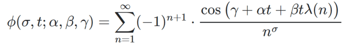
with 0 < σ < 1, t a real number, α, β, γ three real parameters, and λ(⋅) a real-valued function with logarithmic growth. Elementary computations show that s = σ + it is a complex root (also called zero) of ζ(s), with 0 < σ < 1, if and only if
- ϕ(σ, t; 0, 1, 0) = 0,
- ϕ(σ, t; 0, 1, −π/2) = 0,
- λ(n) = log(n).
For details about this formulation, see here. Moving forward, we will focus on RH as being a problem of finding the zeroes (or lack of) of a bivariate function in the standard plane: σ is the first variable, attached to the X-axis, and t is the second variable, attached o the Y-axis. A generalized version of RH seems to also be true: it corresponds to arbitrary values for α, β, γ. However we focus here on the classical RH. For ease of presentation, we use the following notation:
- ϕ1(σ, t) = ϕ(σ, t; 0, 1, 0)
- ϕ2(σ, t) = ϕ(σ, t; 0, 1,−π/2 )
Much of the discussion has to do with the orbit of (ϕ1, ϕ2) when σ is fixed but arbitrary, and only t is allowed to vary. The orbit consists of all the points (X(t), Y(t)) with X(t) = ϕ1(σ, t) and Y(t) = ϕ2(σ, t). In short, we are dealing with a bivariate time series in continuous time, with strong cross-correlations between X(t) and Y(t). Without loss of generality, we assume that t is positive. The spectacular plot shown in section 2 is just a scatterplot of the orbit, computed for σ = 0.75. It easily generalizes to other values of σ that are strictly greater than 0.5.
2. The visualization
I call the plot below the Eye of the Zeta Function. It is the scatter plot described in the last paragraph in section 1, and probably the first time that such a plot was created for the Riemann zeta function. It corresponds to σ = 0.75, with t between 0 and 3,000, with t increments equal to 0.01. Thus 300,000 points of the orbit are displayed here.
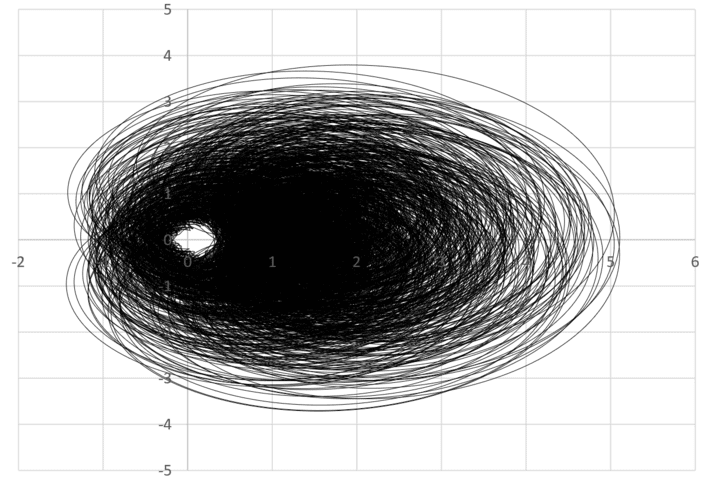
The spectacular feature in that plot is the hole around (0, 0). It has deep implications. It suggests that if σ = 0.75, not only ϕ1(σ, t) and ϕ2(σ, t) can not be simultaneously equal to zero (this is a particular case of RH, nothing new here), but most importantly, that it never jointly gets very close to zero. This is new and suggests that proving RH might be a little less challenging than initially thought. The same plot features a similar “eye” if you try various values of σ. In particular, the hole gets smaller and smaller as σ gets closer to 0.5. At σ = 0.5, the hole is entirely gone, and infinitely many values of t yield ϕ1(σ, t) = ϕ2(σ, t) = 0. The same is true for a generalized version of RH discussed in section 1.
Note that it is very tricky to get the scatterplot right. The series for ϕ1 and ϕ2 converge very slowly, and in chaotic, unpredictable way, see here. This can result in false positives: points very close to zero due to approximation errors, artificially obfuscating the hole. Convergence boosting techniques are required, see here. In addition, the frequency of oscillations in ϕ1 and ϕ2 increases more and more as t gets larger, and thus t increments should be made smaller and smaller accordingly, as t grows, in order to get a good coverage of the orbit and not miss potential true zeroes.
More plots can be found here. One (unpublished yet) is even more spectacular, though esthetically speaking, it looks just like a boring ring. I computed the approximation error (E1(t), E2(t)) when you use only the first 200 terms in the series defining ϕ1 and ϕ2. If t < 300, these points are located on a very thin ring very close to 0. Their distribution thus has a strong pattern, making it possibly even less challenging to prove that if σ = 0.75, then the Riemann Zeta function has no zero with t in [0, 300]. The pattern quickly disappears if t is larger, but you can still retrieve it by increasing the number of terms that you use in your approximation, allowing you to identify an even bigger zero-free zone in the critical strip. Proving it is zero-free even narrowed down to these zones, would still remain a big challenge though.
About the author: Vincent Granville is a data science pioneer, mathematician, book author (Wiley), patent owner, former post-doc at Cambridge University, former VC-funded executive, with 20+ years of corporate experience including CNET, NBC, Visa, Wells Fargo, Microsoft, eBay. Vincent also founded and co-founded a few start-ups, including one with a successful exit (Data Science Central acquired by Tech Target). You can access Vincent’s articles and books, here.