Simpson’s Paradox, the Bane of Clinical Trials

(This article is now a chapter of my github proto-book Bayesuvius)
Simpson’s paradox is a recurring nightmare for all statisticians overseeing a clinical trial for a medicine. It is possible that if they leave out a certain “confounding” variable from a study, the study’s conclusion on whether a medicine is effective or not, might be, without measuring that confounding variable, the opposite of what it would have been had that variable been measured. Statisticians have to enlist expert knowledge to assure themselves that no influential variables are left out.

Judea Pearl considers Simpson’s Paradox a fundamental problem which is greatly clarified by his theory of causal Bayesian networks (See references below).

Here is a simple example of Simpson’s Paradox (Or Simpson’s curse, or Simpson’s weed).

Some patients of both male and female genders are given a medicine or a placebo in a double blind study. Some recover from their ailment and others don’t. Let

r= recovered? No=0, Yes=1

t= took medicine? No=0, Yes=1

g= gender? Female=0, Male=1

The situation can be modeled by the Bayesian Network (bnet) in Fig.1

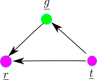
Figure 1

For this bnet, one has

Therefore,
$P(r=1|t)= \sum_g P(r=1|t, g)P(g|t)=E_{\underline{g}|t} P(r=1|t, \underline{g})$

where $E_{\underline{g}|t}$ is a conditional expected value (a kind of weighted average).

Suppose are non-negative real numbers. For the vector $\vec{q}=(q_0, q_1)$ :

Define a positive outcome (or success or increasing with t if $q_0 \leq q_1$ .

Define a negative outcome (or failure or decreasing with t if $q_0 \geq q_1$ .

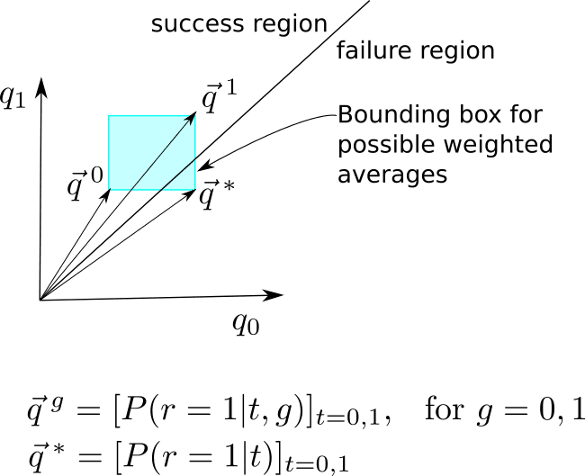
Figure 2

It is possible (see Fig. 2 for a graphical explanation of how) to find perverse cases in which and increase with t but decreases with t. So it is possible to conclude that the medicine is a success for each of the two g populations considered separately, yet the medicine is a failure when both populations are “amalgamated”. The lesson is that a “trend reversal” is possible upon amalgamation. The sign of the outcomes is not necessarily preserved when we do a weighted average of type $E_{\underline{g}|t}$ . $E_{\underline{g}|t}$ is an expected value on the “confounding” random variable g conditioned on the root random variable t.

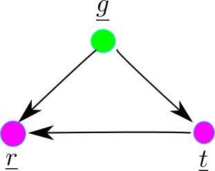
Figure 3

Footnote: Sometimes the bnet Fig.3 is used to explain Simpson’s paradox instead of the bnet Fig.1. But those two bnets are equivalent because

References

“Understanding Simposon’s Paradox”, by Judea Pearl
Simpson’s Paradox: The riddle that would not die. (Comments on four recent papers), by Judea Pearl
“Simpson’s Paradox and the implications for medical trials’, by
Norman Fenton, Martin Neil, Anthony Constantinou,