Model Selection: Adjusted Coefficient of Determination-Variance Tradeoff

In my previous article, we analyzed the COVID-19 data of Turkey and selected the cubic model for predicting the spread of disease. In this article, we will show in detail why we selected the cubic model for prediction and see whether our decision was right or not.

When we analyze the regression trend models we should consider overfitting and underfitting situations; underfitting indicates high bias and low variance while overfitting indicates low bias and high variance.

Bias is the difference between the expected value of fitted values and observed values:

The variance of fitted values is the expected value of squared deviation from the mean of fitted values:

The adjusted coefficient of determination is used in the different degrees of polynomial trend regression models comparing. In the below formula p denotes the number of explanatory terms and n denotes the number of observations.

SSE is the residual sum of squares:

SST is the total sum of squares:

When we examine the above formulas, we can notice the similarity between SSE and bias. We can easily say that if bias decreases, SSE will decrease and the adjusted coefficient of determination will increase. So we will use the adjusted R-squared instead of bias to balance with variance and find the optimal degree of the polynomial regression.

The dataset and data frame(tur) we are going to use can be found from the previous article. First of all, we will create all the polynomial regression models which we’re going to compare.

a <- 1:15 models <- list()  
for (i in seq_along(a)){      
models[[i]] <-  assign(paste0('model_', i),lm(new_cases ~ poly(index, i), data=tur))      
 }

The variances of fitted values of all the degrees of polynomial regression models:

variance <- c()  
for (i in seq_along(a)) {      
variance[i] <- mean((models[[i]][["fitted.values"]]-mean(models[[i]][["fitted.values"]]))^2)    
 }

To create an adjusted R-squared object we first create a summary object of the trend regression models; because the adj.r.squared feature is calculated in summary function.

models_summ <- list() 
adj_R_squared <- c() 
for (i in seq_along(a)) {
 models_summ[[i]] <- summary(models[[i]])   
 adj_R_squared[i] <- (models_summ[[i]][["adj.r.squared"]]) 
 }

Before analyzing numeric results of variance and adjusted R-squared we will show all the trend regression lines in separate plots for comparing models.

# Facetting models by degree for finding the best fit

library(ggplot2)  
 dat <- do.call(rbind, lapply(1:15, function(d) {  
 x <- tur$index  
 preds <- predict(lm(new_cases ~ poly(x, d), data=tur), newdata=data.frame(x=x))   
 data.frame(cbind(y=preds, x=x, degree=d)) }))  
 
 ggplot(dat, aes(x,y)) +   
 geom_point(data=tur, aes(index, new_cases)) +   
 geom_line(color="steelblue", lwd=1.1)+  
 facet_wrap(~ degree,nrow = 3)

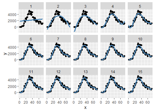
When we examine the above plots, we should pay attention to the curved of the tails; because it indicates overfitting which shows extreme sensitivity to the observed data points. In light of this approach, the second and third-degree of models appear to be more convenient to the data.

Let’s examine the adjusted R-squared-variance tradeoff on the plot we created below.

library(gridExtra) 

plot_variance <- ggplot(df_tradeoff,aes(degree,variance))+  
 geom_line(size=2,colour="orange")+  
 scale_x_continuous(breaks = 1:15)+  
 theme_bw(base_line_size = 2) 
 
 plot_adj.R.squared <- ggplot(df_tradeoff,aes(degree,adj_R_squared))+   
 geom_line(size=2,colour="steelblue")+  
 labs(y="Adjusted R-Squared")+   
 scale_x_continuous(breaks = 1:15)+  
 theme_bw(base_line_size = 2)     
 
 grid.arrange(plot_variance,plot_adj.R.squared,ncol=1) 

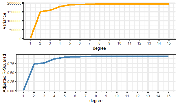
As we can see above, adjusted R-squared and variance have very similar trend lines. The more adjusted R-squared means the more complexity and low bias, but we have to take into account the variance; otherwise, we fall into the overfitting trap. So we need to look for low bias (or high adjusted R-squared) and low variance as much as possible for optimal selection.

When we examine the variance plot, we can see that there is not much difference between second and third-degree; but after the third degree, there seems to be a more steep increase; it’s some kind of breaking. This might lead to overfitting. Thus the most reasonable option seems to be the 3rd degree. This approach is not a scientific fact but could be used for an optimal solution.

Original post can be viewed here