
Regularization And Its Types
Hello Guys, This blog contains all you need to know about regularization. This blog is all about mathematical intuition behind regularization and its Implementation in python.This blog is intended specially for newbies who are finding regularization difficult to digest. For any machine learning enthusiast , understanding the mathematical intuition and background working is more important then just implementing the model.
I am new to world of blogging so If anyone encounters any problem whether conceptual or language-related please comment below. Back in the days, when I came across regularization it became difficult for me to to get mathematical intuition behind it.
I came across many blogs which were answering why regularization is needed and what it does but failed to answer how?
Regularization helps to avoid overfitting so the first question comes to mind is :
What is Overfitting?
Each dataset comprises of some amount of noise. When your model tries to fit your data too well then you crash
into overfitting. Overfitting tries to reach every noise data thus increases complexity. The repercussions of overfitiing is that your model’s training accuracy will be too high whereas testing accuracy will be too low. This means that your model will fail to predict new data.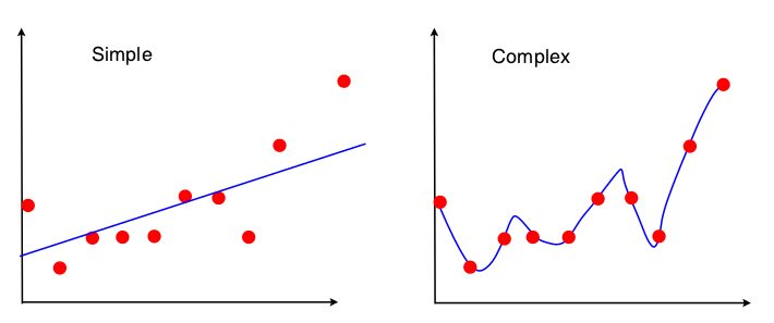 The figure on the right represents Overfitting. One way of avoiding overfitting is to penalize the weights/coefficients
and this is exactly what regularization does.
Regularization
It is a form of regression, that constrains or shrinks the coefficient estimating towards zero. In other words, this technique discourages learning a more complex or flexible model, so as to avoid the risk of overfitting.
There are mainly two types of regularization:
1. Ridge Regression
I’ll explain generalized mathematical intuition by taking ridge regression into context which would be further same for other types except the regularization term. Imagine you’re working on simple linear regression.
So, the formula for hypothesis would be:
h(x) = theta0 + theta1 *x
h(x) –> Predicted Value
y–>Actual Value
m –> Total number of Training examples
n –> Total number of features
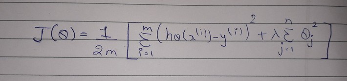
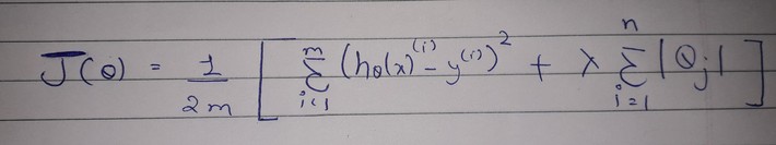
Here, J(theta ) is the cost function for a model. It is different from normal cost function as regularization term is added to penalize the coefficients in the end. Lambda is regularization rate.
Here. Regularization term is lamdba multiplied to the summation of square of coefficients. Therefore adding regularization term, increases cost function as compared to normal cost function
Note: Normal cost function is the same as shown in above figure but doesn’t have regularization term So don’t get confused.
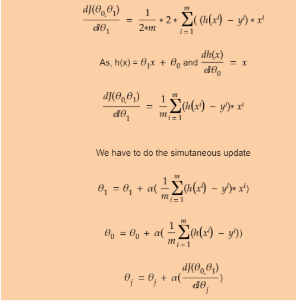
In each model after computing cost we use any optimizing algorithm to improve our weights. In this case we’ll use gradient descent for optimization.
Gradient Descent is a process to find optimal weights/coefficient which is turn used to predict new samples/data.
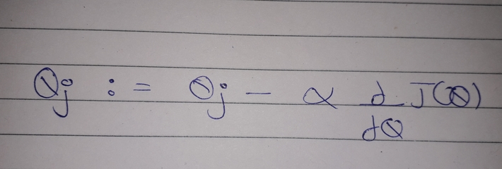
In Gradient Descent, new weights are obtained when learning rate (alpha) is multiplied with derivative(differentiation) of cost function and deducted from old weight. This process occurs for multiple iterations where weights are optimized simultaneously.
As we saw earlier that adding regularization term increases cost function so when derivative of cost function is deducted from weights in gradient descent then new weights would be much more lesser as compared to that we obtained using normal cost function(without regularization).
In simple words, if cost function without regularization is termed as X and cost function with regularization is termed as Y then it is obvious that Y>X as regularization term is added. Also new weights computed using cost function with regularization is W1 and new weights computed using cost function without reqularization is W2 then W2>W1.
 \
\
.
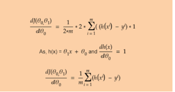
The above two figures shows how gradient descent works in detail. It takes Simple linear Regression as model under consideration.
Coming back to Ridge Regression, Drawback of ridge regressor is that it can reduce the coefficients/weights to minimum threshold but can’t reduce it to zero. Ridge regression is used when multi-collinearity occurs. Multi-collinearity means features are dependent on each other.
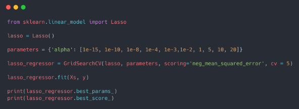
2. Lasso Regression (L1 Regression)
Lasso follows same mathematical intution as stated above in ridge regression. The only difference is in regularization term. Regularization term is regularization rate multiplied with summation of modulus of weights. Lasso Regression overcomes the drawback of ridge regression by not only penalizing the coefficients but also setting them to zero if not relevant to dependent variable.
So, Lasso regression can also be used as feature selection and it comes under embedded methods of feature selection.
Python Implementation
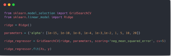
****This code only shows implementation of model.****
Steps:
1. Import library
2. Create an object of the function (ridge and lasso)
3. Fit the training data into the model and predict new ones.
Here, alpha is the regularization rate which is induced as parameter.
How to use Regularization Rate ?
On implementing any of these regression techniques If you are facing :
(1) Overfitting –> Try to increase the regularization rate.
(2) Underfitting –> Try to decrease the regularization rate.
End Notes
In this article we got a general understanding of regularization. In reality the concept is much deeper than this.
Did you find the article useful? Do let us know your thoughts about this article in the comment box below.
That’s all folks, Have a nice day 🙂