The Mathematics of Data Science: Understanding the foundations of Deep Learning through Linear Regression

Note: This is a long post, but I kept it as a single post to maintain continuity of the thought flow

In this longish post, I have tried to explain Deep Learning starting from familiar ideas like machine learning. This approach forms a part of my forthcoming book. You can connect with me on Linkedin to know more about the book. I have used this approach in my teaching. It is based on ‘learning by exception,' i.e. understanding one concept and it’s limitations and then understanding how the subsequent concept overcomes that limitation.

The roadmap we follow is:

Linear Regression
Multiple Linear Regression
Polynomial Regression
General Linear Model
Perceptron Learning
Multi-Layer Perceptron

We thus develop a chain of thought that starts with linear regression and extends to multilayer perceptron (Deep Learning). Also, for simplification, I have excluded other forms of Deep Learning such as CNN and LSTM, i.e. we confine ourselves to the multilayer Perceptron when it comes to Deep Learning. Why start with Linear Regression? Because it is an idea familiar to many even at high school levels.

Linear Regression

Let us first start with the idea of ‘learning’. In Machine Learning, the process of learning involves finding a mathematical function that maps the inputs to the outputs.

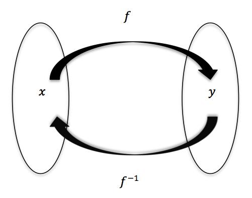
Source: http://www.math.toronto.edu/preparing-for-calculus/4_functions/we_4...

In the simplest case, that function is linear

What is a Linear Relationship?

A linear relationship means that you can represent the relationship between two sets of variables with a straight line. Many phenomena represent a linear relationship. For example, the force involved in stretching a rubber band. We can represent this relationship in the form of a linear equation in the form:

y = mx + b

Where:

“m” is the slope of the line,

“x” is any point (an input or x-value) on the line,

and “b” is where the line crosses the y-axis.

In linear relationships, any given change in an independent variable produces a corresponding change in the dependent variable. Linear regression is used in predicting many problems like sales forecasting, analysing customer behaviour etc.

It can be represented as below:

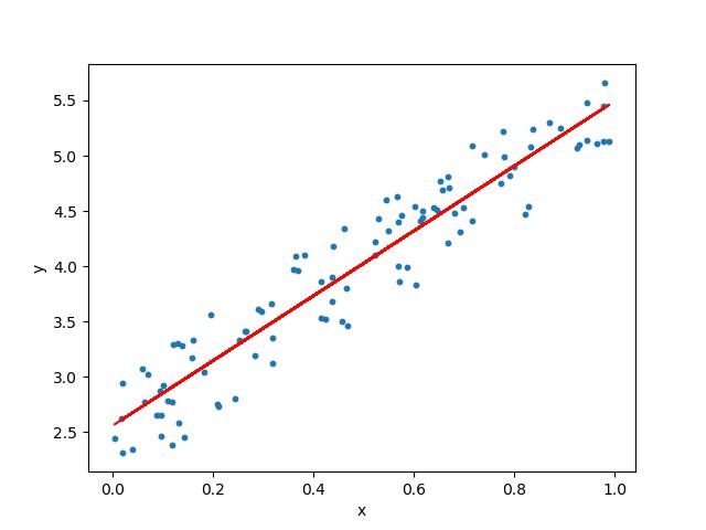
The linear regression model aims to find a relationship between one or more features (independent variables) and a continuous target variable (dependent variable). We refer to the above as Ordinary Linear Regression, i.e. the simplest form of Linear Regression

Let us now consider three models which we can infer from Ordinary Linear Regression

Multiple Linear Regression
Generalised Linear model
Polynomial Regression

1) Multiple Linear Regression

The first obvious variant of the simple Linear Regression is multiple linear regression. When there is only one feature, we have Uni-variate Linear Regression, and if there are multiple features, we have Multiple Linear Regression. For Multiple linear regression, the model can be represented in a general form as

This equation is a more generic form of the equation y = mx + c

Training of the model involves finding the parameters so that the model best fits the data. The line for which the error between the predicted values and the observed values is minimum is called the best fit line or the regression line. These errors are also called as residuals. The residuals can be visualised by the vertical lines from the observed data value to the regression line.

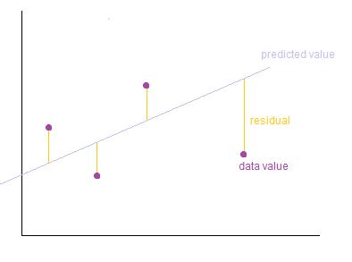
Image Credits: http://wiki.engageeducation.org.au/further-maths/data-analysis/resi...

To define and measure the error of our model we define the cost function as the sum of the squares of the residuals. The cost function is denoted by

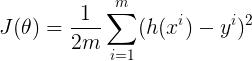
Credits: http://www.wbur.org/radioboston/2013/09/18/bostons-housing-challenge

Multiple linear regression can be illustrated in the commonly used Boston Housing Dataset

The description of the features in the Boston Housing Dataset is as below:

CRIM: Per capita crime rate by town

ZN: Proportion of residential land zoned for lots over 25,000 sq. ft

INDUS: Proportion of non-retail business acres per town

CHAS: Charles River dummy variable (= 1 if tract bounds river; 0 otherwise)

NOX: Nitric oxide concentration (parts per 10 million)

RM: Average number of rooms per dwelling

AGE: Proportion of owner-occupied units built prior to 1940

DIS: Weighted distances to five Boston employment centers

RAD: Index of accessibility to radial highways

TAX: Full-value property tax rate per $10,000

PTRATIO: Pupil-teacher ratio by town

LSTAT: Percentage of lower status of the population

MEDV: Median value of owner-occupied homes in $1000s

The prices of the house indicated by the variable MEDV is the target variable, and the remaining are the feature variables based on which we predict the value of a house.

There are a number of good solutions to the Boston Housing Dataset problem

https://towardsdatascience.com/linear-regression-on-boston-housing-...

https://www.edvancer.in/step-step-guide-to-execute-linear-regressio...

https://www.ritchieng.com/machine-learning-project-boston-home-prices/

https://medium.com/@haydar_ai/learning-data-science-day-9-linear-re...

Training a Multilayer Perceptron to predict the final selling price....

2) Generalised Linear Model

Let us now look at a second model that we can infer from Ordinary Linear Regression, i.e. Generalized Linear Regression. In Ordinary Linear Regression, we can predict the expected value of the response variable (the Y term) as a linear combination of a set of predictors (the X terms). As we have seen before, this implies that a constant change in a predictor leads to a constant change in the response variable. However, this is appropriate only when the response variable has a normal distribution. Normal distributions apply when the response variables change by relatively small amounts around a peak value (for example in the case of human heights).

The requirement that the response variable is of normal distribution excludes many cases such as:

Where the response variable is expected to be always positive and varying over a wide range or
Constant input changes lead to geometrically varying, rather than continually varying, output changes.

We can illustrate these using examples:

Suppose we have a model which predicts that a 10 degree temperature decrease would lead to 1,000 fewer people visiting the beach. This model does not work over small and large beaches. (Here, we could consider a small beach as one where expected attendance is 50 people and a large beach as one where the expected attendance was 10,000.). For the small beach (50 people), the model implies that -950 people would attend the beach. This prediction is obviously not correct
This model would also not work if we had a situation where we had an output that was bounded on both sides – for example in the case of a yes/no choice. This is represented by a Bernoulli variable where the probabilities are bounded on both ends (they must be between 0 and 1). If our model predicted that a change in 10 degrees makes a person twice as likely to go to the beach. As temperatures increase by 10 degrees, probabilities cannot be doubled.

Generalised linear models cater to these situations by

Allowing for response variables that have arbitrary distributions (other than only normal distributions), and
Using an arbitrary function of the response variable (the link function) to vary linearly with the predicted values (rather than assuming that the response itself must vary linearly).

Thus, in a generalised linear model (GLM), each outcome Y of the dependent variables is assumed to be generated from the exponential family of distributions (which includes distributions such as the normal, binomial, Poisson and gamma distributions, among others). GLM uses the maximum likelihood estimation of the model parameters. (Note the section adapted from Wikipedia)

3) Polynomial Regression

Having looked at the Multiple Regression and the GLM, let us now look at another model that we can infer from Ordinary Linear Regression, i.e. Polynomial Regression. Many relationships do not fit the Linear format at all. In polynomial regression, the relationship between the independent variable x and the dependent variable y is modelled as an nth degree polynomial in x. Polynomial regression has been used to describe nonlinear phenomena such as the growth rate of tissues, the distribution of carbon isotopes in lake sediments, and the progression of disease epidemics.

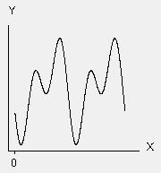
Fourier: Theta1 * cos(X + Theta4) + (Theta2 * cos(2*X + Theta4) + Theta3

Source minitab

References:

http://statisticsbyjim.com/regression/curve-fitting-linear-nonlinea...

http://blog.minitab.com/blog/adventures-in-statistics/linear-or-non...

http://support.minitab.com/en-us/minitab/17/topic-library/modeling-...

https://www.datasciencecentral.com/profiles/blogs/curve-fitting-usi...

Perceptron Learning

Image source: asharperfocus

Just like the Space Odyssey 2001 bone scene – let us now Let us now switch tools to a new model.

However, we show how these new tools and old tools are related. We now consider a new model called Perceptron learning, and we show how it relates to Linear Regression.

The perceptron is an algorithm for supervised learning of binary classifiers. an input, represented by a vector of numbers, belongs to some specific class. Binary classifiers are a type of linear classifier for two classes.

Perceptrons started off being implemented in hardware. The Mark I Perceptron machine was the first implementation of the perceptron algorithm. The perceptron algorithm was invented in 1957 at the Cornell Aeronautical Laboratory by Frank Rosenblatt. The perceptron was intended to be a machine, rather than a program. This machine was designed for image recognition: it had an array of 400 photocells, randomly connected to the "neurons". Weights were encoded in potentiometers, and weight updates during learning were performed by electric motors. There was misplaced optimism about perceptrons. In a 1958 press conference organized by the US Navy, Rosenblatt made statements about the perceptron that caused a heated controversy among the fledgeling AI community; based on Rosenblatt's statements, The New York Times reported the perceptron to be "the embryo of an electronic computer that [the Navy] expects will be able to walk, talk, see, write, reproduce itself and be conscious of its existence."

Although the perceptron initially seemed promising, it was quickly proved that perceptrons could not be trained to recognise many classes of patterns. This misplaced optimism caused the field of neural network research to stagnate for many years before it was recognised that a feedforward neural network with two or more layers (also called a multilayer perceptron) had far greater processing power than perceptrons with one layer (i.e. single layer perceptron). Single layer perceptrons are only capable of learning linearly separable patterns. In 1969, a famous book entitled Perceptrons by Marvin Minsky and Seymour Papert showed that it was impossible for these classes of network to learn an XOR function.

However, this limitation does not apply if we use a non-linear activation function (instead of a step function) for a perceptron. In fact, by using non-linear activation functions, we can model many more complex functions than the XOR (even with just the single layer). This idea can be extended if we add more hidden layers – creating the multilayer perceptron.

So, to recap:

The perceptron is a simplified model of a biological neuron.
The perceptron is an algorithm for learning a binary classifier: a function that maps its input to an output value (a single binary value).
In the context of neural networks, a perceptron is an artificial neuron using the Heaviside step function as the activation function. The perceptron algorithm is also termed the single-layer perceptron, to distinguish it from a multilayer perceptron.
While the Perceptron algorithm is of historical significance, it provides us with a way to bridge the gap between Linear Regression and Deep Learning.
Below is an example of a learning algorithm for a (single-layer) perceptron. A diagram showing a perceptron updating its linear boundary as more training examples are added.

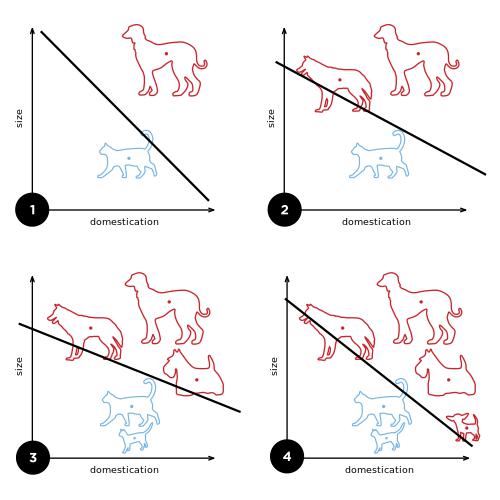
Image source Wikipedia

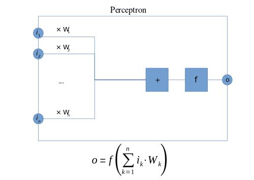
A preceptron is represented as above. Here, f is a step function. As we have seen before, a perceptron takes several binary inputs, x1,x2,…x1,x2,…, and produces a single binary output:

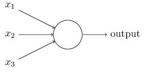
In the example shown the perceptron has three inputs, x1 ,x2, x3 and weights, w1,w2,…w1,w2,…, are real numbers expressing the importance of the respective inputs to the output. The neuron's output, 0 or 1, is determined by whether the weighted sum ∑jwjxj is less than or greater than some threshold value. A way you can think about the perceptron is that it's a device that makes decisions by weighing up evidence. This idea is similar to the Multiple linear equation we have seen before

Multi-Layer Perceptron

We now come to the idea of the Multi-layer perceptron(MLP). Multilayer perceptrons overcome the limitations of the Single layer perceptron by using non-linear activation functions and also using multiple layers. The MLP needs a combination of backpropagation and gradient descent for training.

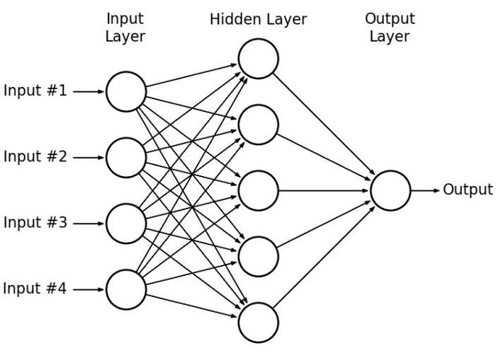
In contrast to a single perceptron, MLPs when seen as a complex network of perceptrons (with non-linear activation functions), could make subtle and complex decisions based on weighing up evidence hierarchically

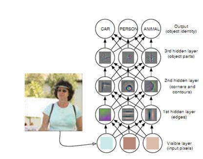
This leads us to the image above from the Deep Learning book by Goodfellow , Bengio , Courville which shows how a hierarchy of layers of neurons can make a decision.

Thus, a neural network (i.e. a multilayer perceptron) with a single layer no activation function (or a step activation function) is equivalent to linear regression. Also, Linear Regression can be solved using a closed form solution. However, with the more complex architecture of the MLP, a closed form solution does not work. Hence, an iterative solution has to be used, i.e. an algorithm that improves the result through a step-wise improvement. Such an algorithm does not necessarily converge – so we are interested in finding a minima. Gradient descent is an example of such an algorithm. References: Closed form vs Gradient Descent

Deep Learning – a highly parameterised model

One final aspect of the model we can infer is – MLP (Deep Learning) is an example of a highly parameterised model. Considering our example of finding the price of a house based on a set of features, for the equation y = mx + c, the quantities m and c are called the parameters. We derive the value of the parameters from the data and the strategy for solving the equation. The parameters of an equation can be seen as the degrees of freedom. Linear regression has a relatively smaller number of parameters. However, the more complex MLP has a much wider range of parameters (degrees of freedom). Both are parameterised models, but MLPs follow a more complex optimisation strategy (back propagation and gradient descent) than Linear Regression (least square)

In this sense, neural networks can be seen as a complex evolution of linear regression. The highly parameterised nature of multilayer perceptrons allow for the modelling of complex functions. I discuss the training of Deep Learning networks in a previous post – a simplified explanation of the mathematics of deep learning