
Many statistics, such as correlations or R-squared, depend on the sample size, making it difficult to compare values computed on two data sets of different sizes. Here, we address this issue.
Below is an example with 20 observations. The 10 last observations (the second half of the data set) is a mirror of the first 10, and the two correlations, computed on each subset, are identical and equal to 0.30. The full correlation computed on the 20 observations is 0.85.
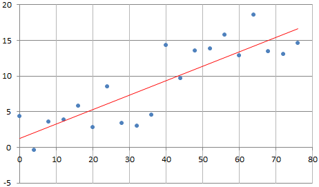
One would expect that since they represent the same association, these correlations should be identical. Of course, by doubling the number of observations (from 10 to 20) you get more statistical significance, and it strengthens the correlation. So from a statistical point of view, it makes sense that the correlation changes (increases) when adding new observations, if the new observations have the same behavior as the previous ones.
But it makes it impossible to make meaningful comparisons between data sets of different sizes. One way around this is to compute correlations on subsets of 10 points. There are 92,378 different ways to select 10 distinct observations out of 20, and thus 92,378 potential correlation values. If you average these values, you will get a number that you can truly be compared with that from a data set of size 10, yet it involves all the 20 observations.
In this case we simply averaged the 10 correlation values computed on all 10 subsets consisting of 10 consecutive observations. The final correlation, you can call it the re-sampled correlation, is equal to 0.67. Now you are no longer comparing apples and oranges.
Using the same data generation mechanism (that is, the same statistical model), I performed ten tests, each time with 20 observations, with the second half of the data set having the same correlation as the first half. This correlation is listed in the third column in the table below. The second column represents the correlation computed on the whole data set (20 observations) while the last (fourth) column represents the re-sampled correlation.
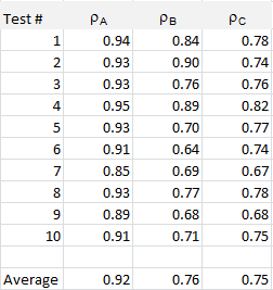
The data, computations, and chart, is available in this spreadsheet. The data set consists of two variables stored in columns C and D. The same methodology could be applied to any coefficient, for instance the R-squared or the regression coefficients in a linear model. More about re-sampling techniques can be found here. For another related trick, follow this link.
To not miss this type of content in the future, subscribe to our newsletter. For related articles from the same author, click here or visit www.VincentGranville.com. Follow me on on LinkedIn, or visit my old web page here.