
Fermat’s last conjecture has puzzled mathematicians for 300 years, and was eventually proved only recently, see here. Some people claim to have found elementary proofs, see here, here, and here. In this note, I propose a generalization, that could actually lead to a much simpler (albeit non-elementary) proof and a more powerful result with broader applications, including to solve numerous similar equations. As usual, my research involves a significant amount of computations and experimental math, as an exploratory step before stating new conjectures, and eventually trying to prove them. The methodology is very similar to that used in data science, involving the following steps:
- Identify and process the data. Here the data set consists of all real numbers; it is infinite, which brings its own challenges. On the plus side, the data is public and accessible to everyone, though very powerful computation techniques are required, usually involving a distributed architecture.
- Data cleaning: in this case, inaccuracies are caused by no using enough precision; the solution consists of finding better / faster algorithms for your computations, and sometimes having to work with exact arithmetic, using Bignum libraries.
- Sample data and perform exploratory analysis to identify patterns. Formulate hypotheses. Perform statistical tests to validate (or not) these hypotheses. Then formulate conjectures based on this analysis.
- Build models (about how your numbers seem to behave) and focus on models offering the best fit. Perform simulations based on your model, see if your numbers agree with your simulations, by testing on a much larger set of numbers. Discard conjectures that do not pass these tests.
- Formally prove or disprove retained conjectures, when possible. Then write a conclusion if possible: in this case, a new, major mathematical theorem, showing potential applications. This last step is similar to data scientists presenting the main insights of their analysis, to a layman audience.
The motivation in this article is two-fold:
- Presenting a new path that can lead to new interesting results and theoretical research in mathematics (yet my writing style and content is accessible to the layman).
- Offering data scientists and machine learning / AI practitioners (including newbies) an interesting framework to test their programming, discovery and analysis skills, using a huge (infinite) data set that has been available to everyone since the beginning of times, and applied to a fascinating problem.
1. New approach to the problem
We are interested in solving
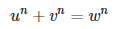 where u, v, w > 0 are integers, and n > 2 is an integer. We start with the following generating function:
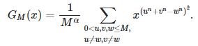
where α ≥ 0. This function has a Taylor series expansion:
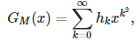
where h(k) is the number of ways (combinations of u,v,w) that k can be written as k = u^n + v^n − w^n.
1.1. Examples
We know that if n > 2, then h(0) = 0 regardless of M (that’s Fermat’s Last Theorem.) If n = 3, α = 0 and M = 100, then h(1) = 4, as we have
- | 6^3 + 8^3 − 9^3 | = 1
- | 8^3 + 6^3 − 9^3 | = 1
- | 9^3 + 10^3 − 12^3 | = 1
- | 10^3 + 9^3 − 12^3 | = 1
If n = 3, α = 0 and M = 200, then h(1) = 12: in addition to the four previous solutions, we also have
- | 64^3 + 94^3 − 103^3 | = 1
- | 94^3 + 64^3 − 103^3 | = 1
- | 71^3 + 138^3 − 144^3 | = 1
- | 138^3 + 71^3 − 144^3 | = 1
- | 73^3 + 144^3 − 150^3 | = 1
- | 144^3 + 73^3 − 150^3 | = 1
- | 138^3 + 175^3 − 172^3 | = 1
- | 175^3 + 138^3 − 172^3 | = 1
1.2. Standardized generating function
If h(1) tends to infinity as M tends to infinity and the growth follows a power law — that is, h(1) = O(M^α) — then we must have α ≠ 0. Note that h(2) could follow a power low with a different α, this is a tricky problem. But at first glance, there seems to be enough smoothness in the way growth occurs among h(0), h(1), h(2) and so on, so that it is possible to find a suitable candidate for α. Indeed a simple rule consists in choosing α such that we always have

I call this the standardized form.
1.1. Reformulation of Fermat’s last theorem
First, let define G(x) as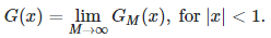
The convergence of this limit is not difficult to establish, but it is beyond the scope of this article. As a result, we have:
Theorem: Fermat’s equation (the first formula in this article, that is, u^n + v^n = w^n), with 0 < u, v, w ≤ M, has no trivial solution (for a specific value of n) if and only if G(0) = 0.
Under this framework, solving Fermat’s problem is equivalent to studying the generating function G associated with the equation in question, around the value x = 0. Not only this methodology applies to many other similar equations (called Diophantine equations), but in addition, it allows you to further explore “almost-solutions” and their statistical distribution, that is, values of u, v, w resulting in h(1) or h(4) being strictly positive, or in other words, almost satisfying the Diophantine equation in question.
2. Interesting facts about the generating function
The values of h(k), for M = 50, 100, 200, 400, 800, 1600, with n = 3 and α = 0, are displayed in the table below:
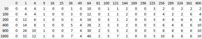
Note that the case n = 2 leads to a singularity, and G does not exist if n = 2, at least not with α = 0 (but maybe with α = 1). Also n can be a real number, but it must be larger than 2. For instance, it seems that n = 2.5 works, in the sense that it does not lead to a singularity for G. Also, we are only interested in x close to zero, say −0.5 ≤ x ≤ 0.5. Finally, G(x) is properly defined (to be proved, may not be easy!) if |x| < 1 and n > 2. If n is not an integer, there is no Taylor approximation for GM, as the successive powers in the Taylor expansion would be positive real numbers, but not integers (in that case it means GM(x) is defined only for 0 ≤ x < 1.)
Below is the plot for GM(x) with −0.5 < x < 0.5, n = 3, α = 0 and M = 200.
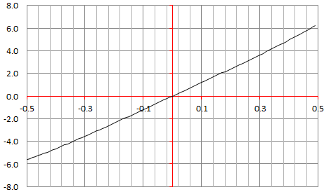
Note that as M tends to infinity, the function GM tends to a straight line around x = 0, with G(0) = 0. This suggests that if there are solutions to u^n + v^n = z^n, with n=3, then the number of solutions must be o(M). The same is true if you plot the same chart for any n > 2. Of course, this assumes that G does not have a singularity at x = 0. Also, if some (u, v, w) is a solution, any multiple is also a solution: so the number of solutions should be at least O(M) in that case. This suggests that indeed, no solution exists.
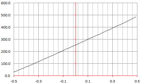
By contrast, the plot below corresponds to n = 2, α = 0, M = 200. Clearly, GM(0) > 0, proving that u^2 + v^2 = w^2 has many, many solutions, even for 0 < u, v, w ≤ 200.
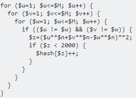
3. Source code
Below is the source code (Perl) used to compute GM. It is easy to implement it in a distributed environment. Here $u**$n means u at power n.
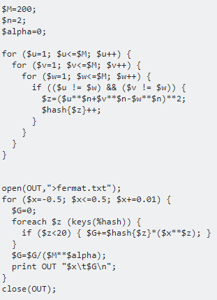
This code is running very slowly because it generates a huge hash table. If we are only interested in the first few coefficients h(k)’s, then the following change in the triple loop significantly improves the speed of the calculations:
The source code is available here.
For more math-oriented articles, visit this page (check the math section), or download my books, available here.