In this article, we show that the issue with polynomial regression is not over-fitting, but numerical precision. Even if done right, numerical precision still remains an insurmountable challenge. We focus here on step-wise polynomial regression, which is supposed to be more stable than the traditional model. In step-wise regression, we estimate one coefficient at a time, using the classic least square technique. 

Even if the function to be estimated is very smooth, due to machine precision, only the first three or four coefficients can be accurately computed. With infinite precision, all coefficients would be correctly computed without over-fitting. We first explore this problem from a mathematical point of view in the next section, then provide recommendations for practical model implementations in the last section. 

This is also a good read for professionals with a math background interested in learning more about data science, as we start with some simple math, then discuss how it relates to data science. Also, this is an original article, not something you will learn in college classes or data camps, and it even features the solution to a regression problem involving an infinite number of variables.

1. Polynomial regression for Taylor series

Here we show how the mathematical machinery behind polynomial regression creates big challenges, even in a perfect environment where the response is well behaved and the exact theoretical model is known. In the next section, we shall show how these findings apply in the context of statistical polynomial regression, to design a better modeling tool for data scientists and statisticians.

Let us consider a function f(x) that can be represented by a Taylor series:

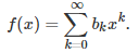
Here we assume that the coefficients are bounded, though the theory also works with a less restrictive assumption, provided that the coefficients do not increase too fast. In most cases, for instance the exponential function, the successive coefficients actually get closer and closer to 0, guaranteeing convergence at least when |x| < 1. The function f(x) does not need to be differentiable; it could even be differentiable nowhere, such as for the Weierstrass function. So the context here is more general than the standard Taylor series framework. 

Stepwise polynomial regression: algorithm

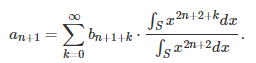
We introduce here an iterative algorithm to estimate the coefficients b(k) one at a time, in the above Taylor series. Note that we are dealing with a regression problem with an infinite number of variables. It is still solved using classic least square approximations. We focus on values of x that are located in a small symmetrical interval centered at 0. This interval is denoted as S. The estimated coefficients are denoted as a(k). We introduce the following notations:

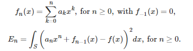
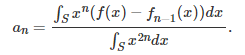
Here, E(n) is called the mean squared error after estimating n coefficients. It measures how well we are approaching the target function f(x) after n steps. The coefficient a(n) (the estimated value of b(n)) is chosen to minimize the mean squared error E(n) in the above formula. Note that the mean squared error is a decreasing function of n. We proceed iteratively starting with n = 0.  As in the standard least square framework, take the derivative of E(n) with respect to a(n), and find its root, to determine a(n). The result is 

Convergence theorem

We have the following remarkable result:

As the interval S, centered at 0, gets smaller and smaller and tends to S = {0}, the estimated coefficients a(k) tend to the true value b(k).

For instance, if f(x) = exp(x), that is, if b(k) = 1 / k!, then the estimates a(k) also tend to 1 / k!. Thus this framework provides an alternate way to compute  the coefficients of a Taylor series, even when derivatives of f(x) do not exist. It also means that step-wise regression, in this context, works just as well as a full-fledged regression, yet involves far fewer computations. A full-fledged regression would involve inverting an infinite matrix. 

The proof of this theorem is quite simple, and proceeds by induction. First, check that a(0) = b(0). Then, if a(k) = b(k) for all k less than or equal to n, we must also have a(n+1) = b(n+1). In order to prove this, note that under this assumption, we have:

As S tends to {0}, all terms except the first one (corresponding to k = 0) in the above series, vanish. Thus a(n+1) = b(n+1), at the limit. Thus, all estimated coefficients match the true ones.

2. Application to Real Life Regression Models

The convergence theorem in the previous section seems to solve everything, even dealing with an infinite number of variables in a regression problem, and yet delivering a smooth, robust theoretical solution to a problem notoriously known for its over-fitting issues. It has to be too good to be true. While the theoretical result is correct, we explore in this section how it translates to applications such as fitting actual data with a polynomial model. It is not pretty, but also not as bad as you would think.

In real life applications, S is your set observations (the independent variable) rather than an interval, after re-scaling these observations so that they are centered at 0, and all very close to 0. You then replace the integral by a sum over all your re-scaled data points. Everything else stays the same.  

I tested this using the same perfectly exponential response f(x) = exp(x), using m = 1,000,000 random deviates  distributed on [-1/m, -1/m] to simulate a real data set. I then computed the estimates a(k). By design, according to the convergence theorem, they should all be close to a(k) = 1 / k!. This did not happen. Indeed it only worked for k = 0 and k = 1. By tweaking the parameters (the set S and m) I was able to get up to four correct coefficients. This is the best that I could get, due to machine precision . Now the good news: Even though higher order coefficients were all very wrong, the impact on interpolation / predictive power was minimal for four reasons:

• S was extremely concentrated around 0,
• As a result, higher terms (k = 3, 4, etc.) had almost no impact on the response,
• As a result, getting higher order estimates a(k), even if totally wrong, had no impact on the error E(n) discussed in the first section,
• It was obvious that beyond k = 3 or k = 4, the error, very small, so small that it was smaller than machine precision, stabilized and did not go up, as expected. 

The most surprising result is as follows, and I noticed this behavior in all my tests:

• Typical values: a(0) = 0.999999995416665, a(1) = 0.999999965249988, a(2) = 3.55555598019368. The correct ones are respectively 1, 1, and 1/2.
• Replace a(0) = 0.999999995416665 by a(0) = 1 in the regression model, now you get a(1) = 1, and a(2) =   0.50000086709697, very close to the theoretical value 1/2. How can such a small difference have such a big impact? 

The answer is because machine precision in standard arithmetic is typically about 15 decimals, and the error E(n) quickly drops to 1 / 10^25, largely because the independent observations are highly concentrated so close to 0. One way to get around this is to use high precision computing. It allows you to work with thousands of correct decimals (or billions if you wanted to, but expect it to be very slow), rather than just 15.  

Recommendations for practical model implementation

Here are some takeaways from my experiments:

• Polynomial regression, in general, should be avoided. If you want to do it, use step-wise polynomial regression as described in this article: it is more stable, and it leads to easier interpretation.
• Re-scale your independent variable, so that all data points for this variable fit in [-1, 1], maybe even in [-0.01, 0.01], to get more robust results. Use for interpolation, not extrapolation.
• Avoid making predictions outside any value of x bigger than 1, or smaller than - 1. 
• Start with a standard linear regression to get your first two estimated coefficients a(0) and a(1) as accurate as possible. Then do a stepwise polynomial regression to get the third and fourth coefficients in your polynomial model, with the first two coefficient estimates set to the value obtained in the linear regression.  
• When the error E(n) does not improve when adding new coefficients and increasing n, stop adding them. This should be your stopping point in your iterative step-wise polynomial regression algorithm, usually occurring at n = 3 or 4 unless you use the techniques (high precision computing and so on) described in this article.

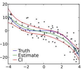
Also, it is easy to compute confidence intervals for the coefficients in the step-wise linear regression, using Monte-Carlo simulations. Add random noise to your data, do it a thousand times with a different noise, and see how the estimated a(k)'s fluctuate based on the added noise: this will help you build confidence bands for your estimates. 

Finally, I've found an article on step-wise polynomial regression, and the author's conclusions are similar to mine. It is entitled Step-wise Polynomial Regression: Royal Road or Detour?, and you can find it here. The conclusion is that we are dealing here with an ill-conditioned problem. In my upcoming research, I will investigate replacing x^k in the Taylor series by a more general term g_k(x). The convergence theorem can easily be generalized, and if I find a suitable function g_k that avoids the issues associated with the polynomial regression, I will share the results.

For related articles from the same author, click here or visit www.VincentGranville.com. Follow me on on LinkedIn.

DSC Resources

• Subscribe to our Newsletter
• Comprehensive Repository of Data Science and ML Resources
• Advanced Machine Learning with Basic Excel
• Difference between ML, Data Science, AI, Deep Learning, and Statistics
• Selected Business Analytics, Data Science and ML articles
• Hire a Data Scientist | Search DSC | Classifieds | Find a Job
• Post a Blog | Forum Questions