Many times, complex models are not enough (or too heavy), or not necessary, to get great, robust, sustainable insights out of data. Deep analytical thinking may prove more useful, and can be done by people not necessarily trained in data science, even by people with limited coding experience. Here we explore what we mean by deep analytical thinking, using a case study, and how it works: combining craftsmanship, business acumen, the use and creation of tricks and rules of thumb, to provide sound answers to business problems. These skills are usually acquired by experience more than by training, and data science generalists (see here how to become one) usually possess them.

This article is targeted to data science managers and decision makers, as well as to junior professionals who want to become one at some point in their career. Deep thinking, unlike deep learning, is also more difficult to automate, so it provides better job security. Those automating deep learning are actually the new data science wizards, who can think out-of-the box. Much of what is described in this article is also data science wizardry, and not taught in standard textbooks nor in the classroom. By reading this tutorial, you will learn and be able to use these data science secrets, and possibly change your perspective on data science. Data science is like an iceberg: everyone knows and can see the tip of the iceberg (regression models, neural nets, cross-validation, clustering, Python, and so on, as presented in textbooks.) Here I focus on the unseen bottom, using a statistical level almost accessible to the layman, avoiding jargon and complicated math formulas, yet discussing a few advanced concepts.   

1. Case Study: The Problem

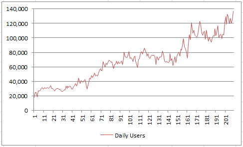
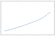
The real-life data set investigated here is a time series with 209 weeks worth of observations. The data points are the number of daily users, averaged per week, for a specific website, over some time period. The data was extracted from Google Analytics, and summarized in the picture below. Some stock market data also shows similar patterns.

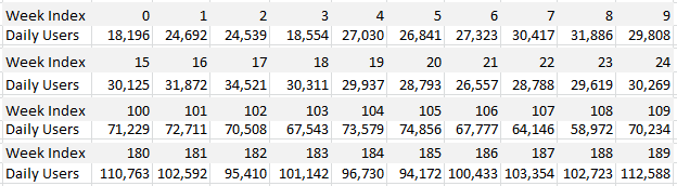
The data and all the detailed computations are available in the interactive spreadsheet provided in the last section. Below is an extract.

Business questions

We need to answer

• whether there is growth over time, in the number of visiting users,
• whether it can be extrapolated to the future (and how),
• what kind of growth do we see (linear, or faster than linear)
• whether can we explain the dips, and avoid them in the future.

As in any business, growth is driven by a large number of factors, as every department tries its best to contribute to the growth. There are also forces going against the growth, such as reaching market saturation, market decline or competition. All the positive and negative forces combine together and can create a stable, predictable growth pattern, either linear, exponential, seasonal, or a combination. This can be approximated by a Gaussian model, by virtue of the central limit theorem. However, in practice, it would be much better to identify these factors to get a much better picture, if one wants to make realistic projections and measure the cost of growth. 

Before diving into original data modeling considerations (data science wizardry) in section 3, including spreadsheets and computations, we first discuss general questions (deep analytical thinking) that should be addressed whenever such a project arises. This is the purpose of the next section. 

2. Deep Analytical Thinking

Any data scientist can quickly run a model and conclude that there is a linear growth in the case discussed in section 1, and make projections based on that. However, this may not help the business if the projections, as we see so frequently in many projects, work for only 3 months or less. A deeper understanding of the opposite forces at play, balancing out and contributing to the overall growth, is needed to sustain the growth. And maybe this growth is not good after all. That's where deep analytical thinking comes in play.

Of course, the first thing to ponder is whether this is a critical business question, coming from an executive wondering about the health of its business (even and especially in good times,) or whether it is a post-mortem analysis related to a specific, narrow, tactical project. We will assume here that it is a critical, strategic question. In practice, data scientists know about the importance of each question, and treat them accordingly with the appropriate amount of deep thinking and prioritization. What I discuss next applies to a wide range of business situations.

Answering hidden questions

It is always good for a data scientist, to be involved in business aspects that are data related, but go beyond coding or implementing models. This is particularly true with small businesses, and it is one aspect of data science that is often overlooked. In bigger companies, this involves working with various teams, as a listener, challenger, and in an advisory role. The questions that we should ask are broken down below in three categories: business, data, and metrics related. 

Business questions:

• Is your company pursuing the correct type of growth? Is it growing in the right segments? Is the growth shifting in the wrong direction? Do we now attract an audience that is not converting well (low ROI) or with high churn rate (low customer lifecycle value, high cost of user acquisition.) The data scientist is well positioned to access the relevant data and analyze it to answer this question. 
• Is top management too much focused on bad growth? That is, growing for the sake of it to show to shareholders? There is good growth and bad growth. In many businesses, some bad growth (growth for the sake of it) is needed to impress clients, shareholders, employees, and because growth numbers from competitors are also fueled partly by bad growth. That is why you want to show that your company is growing as fast as your competition. Good growth, to the contrary, is focused on long terms outcomes. However, now that granular data from most companies is widely available or can be purchased and analyzed by experts, it is becoming more difficult to fake the growth. Anyway, when analyzing statistics, you must be able to discriminate between good and bad growth.
• What external factors impact the bottom line metrics? Competition and market trends are two of them. Knowing that a competitor just received a new round of funding and is spending it on advertising, can be very valuable to gain insights. Or in our example, the big dip corresponds to holiday traffic in December.
• What internal factors are at play and "influencing" your data? It could be increased marketing efforts by your company, a website that was made much more efficient, some business acquisition or new products, the definition of a metric that was changed internally (with impact on measured numbers). The data scientist should be informed about these events, and indeed, proactively ask questions when data trends are seen but can not be explained. Even when data sounds stable, it could be the effect of two sources, one negative, and one positive, canceling out. Always be curious about what is happening in your company, with your competitors and the market in general.

Data questions:

• Are we gathering data from external sources, to validate internal data? In our case, data from Google Analytics can be wrong. Having an external source will help you pinpoint discrepancies and understand what is exactly measured by the various sources. A tool such as Alexa not only provides an alternate source of measurements, but also provide data points about competition.
• Is some data duplicated, missing, corrupt, or not available? Are you working with the IT and BI team to collect the right data, get it properly summarized, accessible via dashboards or straight from databases, and archived appropriately, locally or externally? Do you maintain a data log, that lists all changes to data over time?
• Do you know the biggest mechanisms introducing biases and errors in your data? In our case, Google Analytics is sensitive to smart bots generating artificial traffic, to websites not being tracked or tagged properly, and to new advertising campaigns being launched, introducing shifts in geolocation and traffic quality. Address all these issues with the right people in your company. Sometimes it requires having access to additional data. 

Question about the metrics:

• Are you collecting the most useful metrics? What important metrics are missing or would be useful to have? Do we you enough granularity? Do you focus on the right metrics? New users might be more important than total users. Pageview numbers are easily manipulated by third parties and thus less reliable. Session duration may be meaningless if users spend a lot of time watching videos on your website. A lot of traffic from US is not good if it is from demographic segments not bringing any value. High traffic numbers might not be good if users complain about the poor quality of your content.
• Finding proxy metrics when the exact ones are not available. For instance, zip code data could be used instead of income. When creating web forms, adding mandatory fields could result in more useful databases and better targeting, though changes also impact the data and create back-compatibility issues, making comparisons difficult when analyzing time series.
• A simple question such as the one discussed in section 1, is too generic. You must analyze growth in various segments, and sometimes, you may discover segments that need to shrink rather than grow. For instance, a website that accepts credit card transactions, written in English, might not be appropriate for countries where credit card use is non-existent, or in locales that can sue you because your content is in English rather than in the local, mandatory language.  
• Should you use a longer time window (if available) to get a better picture, assuming the data is consistent over time? Or monthly rather than weekly data? How frequently should this analysis be done? Can it be automated if done frequently enough? Should it be included in dashboard reporting? Which charts to use to communicate the insights visually, with maximum impact and value to the stakeholder?

In the next section, we focus on the modeling aspects, offering different perspectives on how to better analyze the type of data  discussed in our case study.

3. Data Science Wizardry

We focus on the problem and data presented in section 1, providing better ad-hoc alternatives (rarely used in a business setting) to regression modeling. This section is somewhat more technical. 

Even without doing any analysis, the trained eye will recognize a linear trend for the growth, in the time series. Even with the naked eye, you can further refine the model and see three distinct patterns: a steady growth initially, followed by a flat plateau, and then the growth becoming fairly steep at the end. The big dip is caused by the holiday season. At this point, one would think that a mixed, piece-wise model, involving both linear and super-linear growth, represents the situation quite well. It takes less than 5 seconds to come to that conclusion.

The idea to represent the time series as a mixed stochastic process -- a blend of a linear and exponential models, depending on the time period -- is rather original and reminiscent of mixture models. Model blending is also discussed here.However, in this section, we consider a simple parametric model. But rather than traditional model fitting, the technique discussed here is based on simulations, and should appeal to engineering and operations research professionals. It has the advantage of being easy to understand yet robust. 

The idea is as follows, and it will become more clear in the illustration that follows:

Generic algorithm

1. Simulate 100 realizations, also called instances, of a stochastic process governed by a small number of easy-to-interpret parameters, each realization with 209 data points as in the original data set, with same starting and end values as in the observed data (or same mean and variance.) The parameters are set to fixed values.
2. Compute the estimated values (averaged over the 100 simulations) of some business quantities of interest, for instance the number of weeks followed by an increase in users, the average week gap between two increases, the average dip depth and width or number of dips (same with spikes), auto-correlations and so on. These quantities are called indicators. 
3. Compute the error between the indicator values computed on the observed time series, and those estimated on the simulations. 
4. Repeat with a different set of parameters until you get a fit that is good enough. 

A potential improvement, not investigated here, is to consider parameters that change over time, acting as if they were priors in a Bayesian framework. It is also easy to build confidence intervals for the indicators, based on the 100 simulations used for each parameter set. This makes sense with bigger data sets, and it can be done even without being a statistical expert (a software engineer can do it.) 

Illustration with three different models

I tested the following models (stochastic processes) to find a decent fit with the data, while avoiding over-fitting. Thus the models used here have few, intuitive parameters. In all cases, the models were standardized to provide the desired mean and variance associated with the observed time series. The models described below are the base models, before standardization. 

Model #1:

This is a random walk with unequal probabilities, also known as a Markov chain. If we denote the average daily users at week t as X(t), then the model is defined as follows: X(t+1) = X(t) - 1 with probability p, and X(t) = X(t) + 1 with probability 1 - p. Since we observe growth, the parameter p must be between 0 and 0.5. Also, it must be strictly above 0 to explain the dips, and strictly below 0.5 otherwise there would be no growth and no decline (on average), over time. Note that unlike a pure random walk (corresponding to p = 0.5), this Markov chain model produces deviates X(t) that are highly auto-correlated. This is fine because, due to growth, the observed weekly numbers are also highly auto-correlated. A parameter value around p = 0.4 yields the lag-1 auto-correlation found in the data. 

Model #2:

This model is a basic auto-regressive (AR) process, defined as X(t+1) = qX(t) + (1 - q)X(t-1) + D(t), with the parameter q between 0 and 1, and the D(t)'s being independent random variables equal to -1 with probability p, and to +1 with probability 1 - p. It also provides a similar lag-1 auto-correlation in the { X(t) } sequence, but in addition, now the sequence Y(t) = X(t+1) - X(t) also exhibits a lag-1 auto-correlation. Indeed, there is also in the data, a lag-1 auto-correlation in the { Y(t) } sequence. A parameter value around q = 0.8 together with p = 0.4, yields that auto-correlation. Note that with the Markov chain (our first model), that auto-correlation (in the { Y(t) } sequence) would be zero. So the AR process is a better model. An even better model would be an AR process with three parameters. 

Model #3:

The two previous models can only produce linear growth trends. In order to introduce non-linear trends, we introduce a new model which is a simple transformation of the AR process. It is defined as Z(t) = exp(r X(t)), where { X(t) } is the AR process.  In addition to the parameters p and q, it has an extra parameter r. Note that when r is close to zero, it behaves almost as an AR process (after standardization), at least in the short term. 

Results

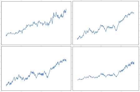
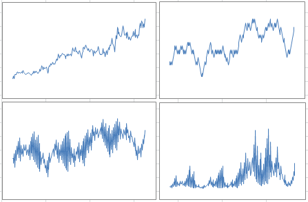
The picture below shows the original data (top left), one realization of a Markov chain with p = 0.4 (top right),  one realization of an AR process with p =0.4 and  q = 0.6 (bottom left), and one realization of the exponential process with p = 0.4, q = 0.6 and r = 0.062. By one realization, we mean any one simulation among the 100 required in the algorithm.

The picture below features the same charts, but with another realization (that is, another simulation) of the same processes, with the same parameter values. Note that the dips and other patterns do not appear in the same order or at the same time, but the intensity, length of dips, overall growth, and auto-correlation structures are similar to those in the first picture, especially if you extend the time window from 209 weeks to a few hundred weeks, for the simulations: they are in the same confidence intervals. If you try many simulations and compute these statistics each time, you will have a clear idea of what these confidence intervals are.

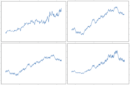
Overall -- when you look at 100 simulations, not just two -- the exponential model with a small value of r, provides the best fit for the first 209 weeks, with a nearly linear growth at least in the short term. However, as mentioned earlier, a piece-wise model would be best. The AR process, while good at representing a number of auto-correlations, seems too bumpy, and dips are not deep enough; a 3-parameter AR process can fix this issue. Finally, model calibration should be performed on test data, with model performance measured on control data. We did not perform this cross-validation step here, due to the small data set. One way to do it with a small data set is to use odd weeks for the test, and even weeks for the control. This is not a good approach here, since we would miss special week-to-week auto-correlations in the modeling process.  

Download the spreadsheet, with raw data, computations, and charts. Play with the parameters!

4. A few data science hacks

Here I share a few more of my secrets.

The Markov chain process can only produce a linear growth. This fact might not be very well known, but if you look at Brownian motions (the time-continuous version of these processes) the expectation and variance over time is well studied and very peculiar, so it can only model a narrow range of time series. More information on this can be found in the first chapters of my book, here. In this article, we overcome this obstacle by using an exponential transformation.

Also growth is usually non-sustainable long-term, and can create bubbles that eventually burst -- one thing that your model may be unable to simulate. One way to mitigate this effect is to use models with constrained growth, in which growth can only go so far and is limited by some thresholds. One such model is presented in my book, see chapter 3 here. 

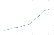
Finally, model fitting is usually easier when you do it on the integrated process (see chapter 2 in my book.) The integrated process is just the cumulative version of the original process, easy to compute, and also illustrated in my spreadsheet. The data / model fit, measured on the cumulative process, can be almost perfect, see picture below representing the cumulative process associated with some simulations performed in the previous sub-section. 

In the above chart, the curve is extremely well approximated by a second-degree polynomial. Its derivative provides the linear growth trend associated with our data. This concept is simple, though I have never seen it mentioned anywhere:

• Use cumulative instead of raw data
• Perform model fitting on the cumulative data
• The derivative of the function (best fit) attached to the cumulative process, provides a great fit with the raw data.

The cumulative function acts as a low-pass filter on the data, removing some noise and outliers. 

Below is another picture similar to those presented earlier, but with a different set of parameter values. It shows that despite using basic models, we are able to accommodate a large class of growth patterns.

And below is the cumulative function associated with the chart in the bottom right corner in the above picture: it shows how smooth it is, despite the chaotic nature of the simulated process. 

In some other simulations (not illustrated here, but you can fine tune the model parameters in the spreadsheet to generate them) the charts present spikes like Dirac distributions, and are very familiar to physicists and signal processing professionals.

To not miss this type of content in the future, subscribe to our newsletter. For related articles from the same author, click here or visit www.VincentGranville.com. Follow me on on LinkedIn, or visit my old web page here.

DSC Resources

• Book and Resources for DSC Members
• New Perspectives on Statistical Distributions and Deep Learning
• Comprehensive Repository of Data Science and ML Resources
• Advanced Machine Learning with Basic Excel
• Difference between ML, Data Science, AI, Deep Learning, and Statistics
• Selected Business Analytics, Data Science and ML articles
• Hire a Data Scientist | Search DSC | Find a Job
• Post a Blog | Forum Questions

Follow us: Twitter | Facebook