
The original version of the central limit theorem (CLT) assumes n independently and identically distributed (i.i.d.) random variables X1, …, Xn, with finite variance. Let Sn = X1 + … + Xn. Then the CLT states that
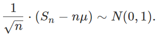
that is, it follows a normal distribution with zero mean and unit variance, as n tends to infinity. Here μ is the expectation of X1.
Various generalizations have been discovered, including for weakly correlated random variables. Note that the absence of correlation is not enough for the CLT to apply (see counterexamples here). Likewise, even in the presence of correlations, the CLT can still be valid under certain conditions. If auto-correlations are decaying fast enough, some results are available, see here. The theory is somewhat complicated. Here our goal is to show a simple example to help you understand the mechanics of the CLT in that context. The example involves observations X1, …, Xn that behave like a simple type of time series: AR(1), also known as autoregressive time series of order one, a well studied process (see section 3.2 in this article).
1. Example
The example in question consists of observations governed by the following time series model: Xk+1 = ρ Xk + Yk+1, with X1 = Y1, and Y1, …, Yn are i.i.d. with zero mean and unit variance. We assume that |ρ| < 1. It is easy to establish the following:
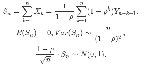
Here “~” stands for “asymptotically equal to” as n tends to infinity. Note that the lag-k autocorrelation in the time series of observations X1, …, Xn is asymptotically equal to ρ^k (ρ at power k), so autocorrelations are decaying exponentially fast. Finally, the adjusted CLT (the last formula above) now includes a factor 1 – ρ. If course if ρ = 0, it corresponds to the classic CLT when expected values are zero.
1.1. More examples
Let X1 be uniform on [0, 1] and Xk+1 = FRAC(bXk) where b is an integer strictly larger than one, and FRAC is the fractional part function. Then it is known that Xk also has (almost surely, see here) a uniform distribution on [0, 1], but the Xk‘s are autocorrelated with exponentially decaying lag-k autocorrelations equal to 1 / b^k. So I expect that the CLT would apply to this case.
Now let X1 be uniform on [0, 1] and Xk+1 = FRAC(b+Xk) where b is a positive irrational number. Again, Xk is uniform on [0, 1]. However this time we have strong, long-range autocorrelations, see here. I will publish results about this case (as to whether or not CLT still applies) in a future article.
1.2. Note
In the first example in section 1.1, with Xk+1 = FRAC(bXk), let Zk = INT(bXk), where INT is the integer part function. Now Zk is the k-th digit of X1 in base b. Surprisingly, if X1 is uniformly distributed on [0, 1], then all the Zk‘s, even though they all depend exclusively on X1, are (almost surely) independent. Indeed, if you pick up a number at random, there is a 100% chance that its successive digits are independent. However, there are infinitely many exceptions, for instance the sequence of digits of a rational number is periodic, thus violating the independence property. But such numbers are so rare (despite constituting a dense set in [0, 1]) that the probability to stumble upon one by chance is 0%. In any case, this explains why I used the word “almost surely”.
2. Results based on simulations
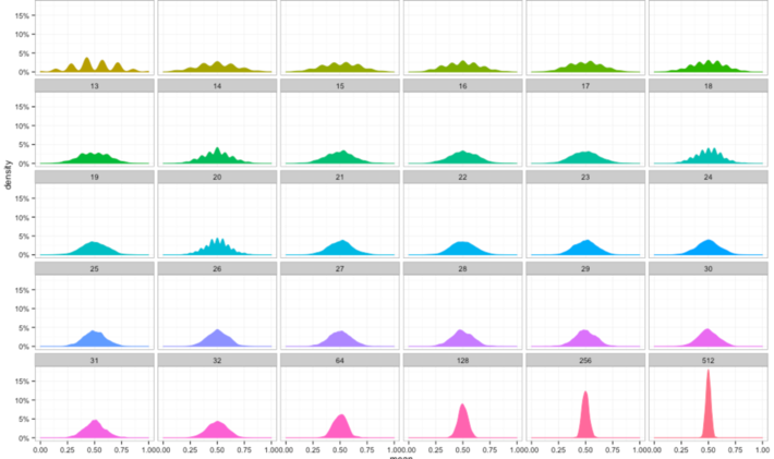
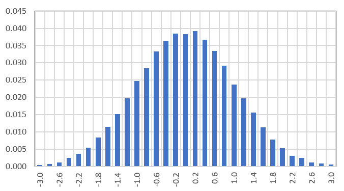
The simulation consisted of generating 100,000 time series X1, …, Xn as in section 1, with Ï = 1/2, each one with n = 10,000 observations, computing Sn for each of them, and standardizing Sn to see if it follows a N(0, 1) distribution. The empirical density follows a normal law with zero mean and unit variance very closely, as shown in the figure below. We used uniform variables with zero mean and unity variance to generate the deviates Yk.
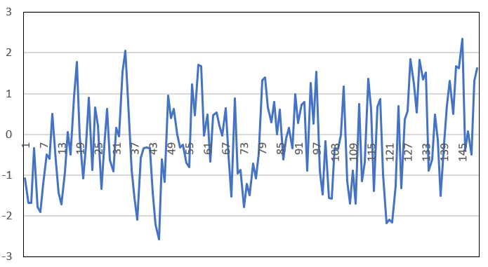
Below is one instance (realization) of these simulated time series, featuring the first n = 150 observations. The Y-axis represents Xk, the X-axis represents k.
The speed at which convergence to the normal distribution takes place has been studied. Typically, this is done using the Berry-Esseen theorem, see here. A version of this theorem, for weakly correlated variables, also exists: see here. The BerryEsseen theorem specifies the rate at which this convergence takes place by giving a bound on the maximal error of approximation between the normal distribution and the true distribution of the scaled sample mean. The approximation is measured by the KolmogorovSmirnov distance. It would be interesting to see, using simulations, if the convergence is slower when Ï is different from zero.
To receive a weekly digest of our new articles, subscribe to our newsletter, here.
About the author: Vincent Granville is a data science pioneer, mathematician, book author (Wiley), patent owner, former post-doc at Cambridge University, former VC-funded executive, with 20+ years of corporate experience including CNET, NBC, Visa, Wells Fargo, Microsoft, eBay. Vincent is also self-publisher at DataShaping.com, and founded and co-founded a few start-ups, including one with a successful exit (Data Science Central acquired by Tech Target). He recently opened Paris Restaurant, in Anacortes. You can access Vincent’s articles and books, here.