
Predictive analysis is heavily used today to gain insights on a level that are not possible to detect with human eyes. And R is an extremely powerful and easy tool to implement the same. In this piece, we will explore how we can predict the status of breast cancer using predictive modeling in less than 30 lines of code.
Who should read this blog?
- Someone who wants to get started with R programming.
- Someone who is new to Machine Learning
Download RStudio: https://www.rstudio.com/products/rstudio/download/
Download the data set (CSV file): https://www.kaggle.com/uciml/breast-cancer-wisconsin-data

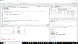
Your RStudio should look like this:
 h
h
You are gonna write your program in the top left box.
What are We About to Do?
Place the downloaded file in a folder. You can name it anything. If you open the CSV file downloaded from Kaggle, it looks something like this –
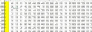
A lot of numbers, right? Those numbers are the features. Features are the attributes of a data point. For example, if a house is a data point, its features could be the carpet is, number of rooms, number of floors, etc. Basically, features describe the data. In our case, the features are a description of the affected breast area. The highlighted column, labeled ‘diagnosis’ is the status of the disease – M for Malignant (dangerous) and B for Benign (not dangerous). This is the variable we wish to predict. It is also called the predicted variable. So we have the features and the predicted variable in our excel sheet. Our task is to train a model that can learn from these labeled (whose diagnosis status is given) points and then can predict for a new data point for which we know the features but not the predicted variable (in this case the ‘diagnosis status’) value.
What Exactly is the Model We Use?
To start with, we use the simplest of all
KNN: K-Nearest Neighbours
“You are the average of 5 people you surround yourself with”-John Rim
Consider a prediction problem. Let’s set K, which is the number of closest neighbours to be considered equal to 3. We have 6 seen data points whose features are height and weight of individuals and predicted variable is whether or not they are obese.
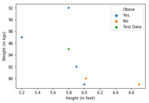
Consider a point from the unseen data (in green). Our algorithm has to predict whether the person represented by the green data point is obese or not. If we consider it’s K(=3) nearest neighbours, we have 2 obese (blue) and one not obese (orange) data points. We take the majority vote of these 3 neighbours which is ‘Yes’. Hence, we predict this individual to be obese.
Easy, right?
The Code
In the console (bottom left box on the RStudio, we first set our working directory. Type in setwd(“//path”) … where the path is the route to your folder. Something like “C:\Users\DHRUVIL\Desktop\R”. Change the \ to / and press enter.
First, we load our data frame –
wbcd<-read.csv(“wisc_bc_data.csv”, stringsAsFactors = FALSE)
The ‘head’ command allows us to view the top few rows (in this case 4) of the dataset. Just to get an idea
head(wbcd,4)
We do not need the ‘id’ column of the data. Hence we drop it using the following command
wbcd<-wbcd[-1]
For our predicted variables, we set the B and M as factors with labels as Benign and Malignant
wbcd$diagnosis<-factor(wbcd$diagnosis, levels = c(“B”,”M”), labels = c(“Benign”,”Malignant”))
Since KNN is a distance-based algorithm, it is a good idea to scale all our numeric features. That way a few features won’t dominate in the distance calculations. We first create a function and then apply that function to all our features (column 2 to 31).
normalize<-function(x)
{
return((x-min(x))/max(x)-min(x))
}
wbcd_n<-as.data.frame(lapply(wbcd[,2:31], normalize))
To implement KNN, we need to install a package called class. In your console, type the following:
install.packages(“class”)
library(“class”)
To check the performance of the model, our data is divided into training and test set. We train the model on the training set and validate the test set.
wbcd_train<-wbcd_n[1:469,]
dim(wbcd_train)
wbcd_test<-wbcd_n[470:569, ]
im(wbcd_test)
wbcd_train_label <- wbcd[1:469,1]
wbcd_test_label <- wbcd[470:569,1]
As you can see, 469 points are used in the training set and the rest in the test set.
Finally, we generate the predictions using
wbcd_pred<-knn(wbcd_train,wbcd_test,wbcd_train_label,k=21)
Here, the model is trained on the wbcd_train and wbcd_train_label and predictions are generated on wbcd_test. The number of neighbors or K is set to 21. The performance of the model is evaluated then.
install.packages(“class”)
library(“class”)
CrossTable(wbcd_test_label,wbcd_pred,prop.chisq = FALSE)
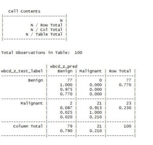
The results are tabulated above. As we can see, out of 77 actual Benign, 0 were misclassified as Malignant. For the 23 actual Malignant, 2 were misclassified as Benign. You can tweak the value of K and check if the results are getting better.
Congratulations on building your first model!
Summary
R is a programming language originally written for statisticians to do statistical analysis, including predictive analytics. It’s open-source software, used extensively in academia to teach such disciplines as statistics, bio-informatics, and economics.
Read more here.