How to Detect if Numbers are Random or Not

In this article, you will learn some modern techniques to detect whether a sequence appears as random or not, whether it satisfies the central limit theorem (CLT) or not — and what the limiting distribution is if CLT does not apply — as well as some tricks to detect abnormalities. Detecting lack of randomness is also referred to as signal versus noise detection, or pattern recognition.

It leads to the exploration of time series with massive, large-scale (long term) auto-correlation structure, as well as model-free, data-driven statistical testing. No statistical knowledge is required: we will discuss deep results that can be expressed in simple English. Most of the testing involved here uses big data (more than a billion computations) and data science, to the point that we reached the accuracy limits of our machines.  So there is even a tiny piece of numerical analysis in this article.

Potential applications include testing randomness, Monte Carlo simulations for statistical testing, encryption, blurring, and steganography (encoding secret messages into images) using pseudo-random numbers. A number of open questions are discussed here, offering the professional post-graduate statistician new research topics both in theoretical statistics and advanced number theory. The level here is state-of-the-art, but we avoid jargon and some technicalities to allow newbies and non-statisticians to understand and enjoy most of the content.  An Excel spreadsheet, attached to this document, summarizes our computations and will help you further understand the methodology used here.

Interestingly, I started to research this topic by trying to apply the notorious central limit theorem (CLT) to non-random (static) variables — that is, to fixed sequences of numbers that look chaotic enough to simulate randomness. Ironically, it turned out to be far more complicated than using CLT for regular random variables. So I start here by describing what the initial CLT problem was, before moving into other directions such as testing randomness, and the distribution of the largest gap in seemingly random sequences.  As we will see, these problems are connected. 

1. Central Limit Theorem for Non-Random Variables

Here we are interested in sequences generated by a periodic function f(x) that has an irrational period T, that is f(x+T) = f(x). Examples include f(x) = sin x with T = 2p, or f(x) = {ax}  where a > 0 is an irrational number, { } represents the fractional part and T = 1/a. The k-th element in the infinite sequence (starting with k = 1) is f(k).  The central limit theorem can be stated as follows:

Under certain conditions to be investigated — mostly the fact that the sequence seems to represent or simulate numbers generated by a well-behaved stochastic process — we would have:

In short, U(n) tends to a normal distribution of mean 0 and variance 1 as n tends to infinity, which means that as both n and m tends to infinity, the values U(n+1), U(n+2) … U(n+m) have a distribution that converges to the standard bell curve.

From now on, we are dealing exclusively with sequences that are equidistributed over [0, 1], thus  m = 1/2 and s = SQRT(1/12). In particular, we investigate f(x) = {ax} where a > 0 is an irrational number and { } the fractional part. While this function produces a sequence of numbers that seems fairly random, there are major differences with truly random numbers, to the point that CLT is no longer valid. The main difference is the fact that these numbers, while somewhat random and chaotic, are much more evenly spread than random numbers.True random numbers tend to create some clustering as well as empty spaces.  Another difference is that these sequences produce highly auto-correlated numbers.

As a result, we propose a more general version of CLT, redefining U(n) by adding two parameters a and b: 

This more general version of CLT can handle cases like our sequences. Note that the classic CLT corresponds to a = 1/2 and b =0. In our case, we suspect that a = 1 and b is between 0 and -1. This is discussed in the next section. 

Note that if instead of f(k), the k-th element of the sequence is replaced by f(k^2) then the numbers generated behave more like random numbers: they are less evenly distributed and less auto-correlated, and thus the CLT might apply. We haven’t tested it yet. 

You will also find an application of CLT to non-random variables, as well as to correlated variables, in my previous article on this topic.

2. Testing Randomness: Max Gap, Auto-Correlations and More

Let’s call the sequence f(1), f(2), f(3) … f(n) generated by our function f(x) an a-sequence. Here we compare properties of a-sequences with those of random numbers on [0, 1] and we highlight the striking differences. Both sequences, when n tends to infinity, have a mean value converging to 1/2, a variance converging to 1/12 (just like any uniform distribution on [0, 1]), and they both look quite random at first glance. But the similarities almost stop here.  

Maximum gap

The maximum gap among n points scattered between 0 and 1 is another way to test for randomness. If the points were truly randomly distributed, the expected value for the length of the maximum gap (also called longest segment) is known and is equal to

See this article for details, or the book Order Statistics published by Wiley, page 135. The max gap values have been computed in the spreadsheet (see section below to download the spreadsheet) both for random numbers and for a-sequences. It is pretty clear from the Excel spreadsheet computations that the average maximum gaps have the following expected values, as n becomes very large:

• Maximum gap for random numbers: log(n) / n as expected from the above theoretical formula
• Maximum gap for a-sequences:  c / n (c is a constant close to 1.5; the result needs to be formally proved)

So a-sequences have points that are far more evenly distributed than random numbers, by an order of magnitude, not just by a constant factor! This is true for the 8 a-sequences (8 different values of a) investigated in the spreadsheet, corresponding to 8 “nice” irrational numbers (more on this in the research section below, about what a “nice” irrational number might be in this context.) 

Auto-correlations

Unlike random numbers, values of f(k) exhibit strong, large-scale auto-correlations: f(k) is strongly correlated with f(k+p) for some values of p as large as 100. The successive lag-p auto-correlations do not seem to decay with increasing values of p. To the contrary, it seems that the maximum lag-p auto-correlation (in absolute value) seems to be increasing with p, and possibly reaching very close to 1 eventually. This is in stark contrast with random numbers: random numbers do not show auto-correlations significantly different from zero, and this is confirmed in the spreadsheet. Also, the vast majority of time series have auto-correlations that quickly decay to 0. This surprising lack of decay could be the subject of some interesting number theoretic research. These auto-correlations are computed and illustrated in the Excel spreadsheet (see section below) and are worth checking out. 

Convergence of U(n) to a non-degenerate distribution

Figures 2 and 3 in the next section (extracts from our spreadsheet) illustrate why the classic central limit theorem (that is, a = 1/2, b =0 for the U(n) formula) does not apply to a-sequences, and why a = 1 and b = 0 might be the correct parameters to use instead. However, with the data gathered so far, we can’t tell whether a = 1 and b = 0 is correct, or whether a = 1 and b = -1 is correct: both exhibit similar asymptotic behavior, and the data collected is not accurate enough to make a final decision on this. The answer could come from theoretical considerations rather than from big data analysis. Note that the correct parameters should produce a somewhat horizontal band for U(n) in figure 2, with values mostly concentrated between -2 and +2 due to normalization of U(n) by design. And a = 1, b = 0, as well as a = 1, b = -1, both do just that, while it is clear that a = 1/2 and b = 0 (classic CTL) fails as illustrated in figure 3. You can play with parameters  a and b in the spreadsheet, and see how it changes figure 2 or 3, interactively. 

One issue is that we computed U(n) for n up to 100,000,000 using a formula that is ill-conditioned: multiplying a large quantity n by a value close to zero (for large n) to compute U(n), when the precision available is probably less than 12 digits. This might explain the large, unexpected oscillations found in figure 2. Note that oscillations are expected (after all, U(n) is supposed to converge to a statistical distribution, possibly the bell curve, even though we are dealing with non-random sequences) but such large-scale, smooth oscillations, are suspicious. 

3. Excel Spreadsheet with Computations

Click here to download the spreadsheet. The spreadsheet has 3 tabs: One for a-sequences, one for random numbers — each providing auto-correlation, max gap, and some computations related to estimating a and b for U(n) — and a tab summarizing n = 100,000,000 values of U(n) for a-sequences, as shown in figures 2 and 3.  That tab, based on data computed using a Perl script, also features moving maxima and moving minima, a concept similar to moving averages, to better identify the correct parameters a and b to use in U(n). 

Confidence intervals (CI) can be empirically derived to test a number of assumptions, as illustrated in figure 1: in this example, based on 8 measurements, it is clear that maximum gap CI’s for a-sequences are very different from those for random numbers, meaning that a-sequences do not behave like random numbers.

Figure 1: max gap times n (n = 10,000), for 8 a-sequences (top) and 8 sequences of random numbers (bottom)

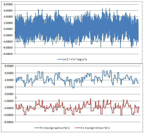
Figure 2: U(n) with a = 1, b = 0 (top) and U(n) moving max / min (bottom) for a-sequences

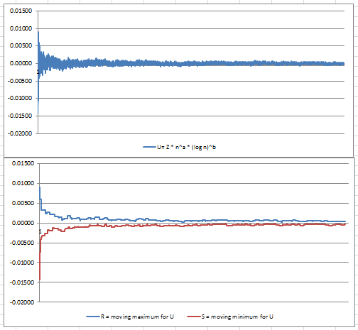
Figure 3: U(n) with a = 0.5, b = 0 (top) and U(n) moving max / min (bottom) for a-sequences

4. Potential Research Areas

Here we mention some interesting areas for future research.  By sequence, we mean a-sequence as defined in section 2, unless otherwise specified. 

• Using f(k^c) as the k-th element of the sequence, instead of f(k). Which values of c > 0 lead to equidistribution over [0, 1], as well as yielding the classic version of CLT with a = 1/2 and b = 0 for U(n)? Also what happens if f(k) = {a p(k)} where p(k) is the k-th prime number and { } represents the fractional part? This sequence was proved to be equidistributed on [0, 1] (this by itself.is a famous result of analytic number theory, published by Vinogradov in 1948) and has a behavior much more similar to random numbers, so maybe the classic CLT applies to this sequence? Nobody knows. 

• What is the asymptotic distribution of the moments and distribution of the maximum gap among the n first terms of the sequence, both for random numbers on [0, 1] and for the sequences investigated in this article? Does it depend on the parameter a? Same question for minimum gap and other metrics used to test randomness, such as point concentration, defined for instance in the article On Uniformly Distributed Dilates of Finite Integer Sequences?

• Does U(n) depend on a? What are the best choices for a, to get as much randomness as possible? In a similar context, sqrt(2)-1 and (sqrt(5)-1)/2 are found to be good candidates: see this Wikipedia article (read the section on additive recurrence.) Also, what are the values of the coefficients a and b in U(n), for a-sequences? It seems that a must be equal to 1 to guarantee convergence to a non-degenerate distribution. Is the limiting distribution for U(n) also normal for a-sequences, when using the correct a and b?

• What happens if a is very close to a simple rational number, for instance if the first 500 digits of a are identical to those of 3/2?

Generalization to higher dimensions

So far we worked in dimension 1, the support domain being the interval [0, 1]. In dimension 2, f(x) = {ax} becomes f(x, y) = ({ax}, {by}) with a, b, and a/b irrational; f(k) becomes f(k,k). Just like the interval [0, 1] can be replaced by a circle to avoid boundary effects when deriving theoretical results, the square [0, 1] x [0, 1] can be replaced by the surface of the torus. The maximum gap becomes the maximum circle (on the torus) with no point inside it. The range statistic (maximum minus minimum) becomes the area of the convex hull of the n points.  For a famous result regarding the asymptotic behavior of the area of the convex hull of a set of n points, read this article and check out the sub-section entitled  “Other interesting stuff related to the Central Limit Theorem.” Note that as the dimension increases, boundary effects become more important. 

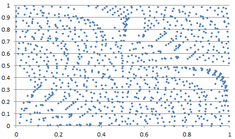
Figure 4: bi-variate example with c = 1/2, a = SQRT(31), b = SQRT(17) and n = 1000 points

Figure 4 shows an unsual example  in two dimensions, with strong departure from randomness, at least when looking at the first 1,000 points. Usually, the point pattern looks much more random, albeit not perfectly random, as in Figure 5

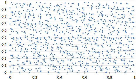. Figure 5: bi-variate example with c = 1/2, a = SQRT(13), b = SQRT(26) and n = 1000 points

Computations are found in this spreadsheet. Note that we’ve mostly discussed the case c = 1 in our article. The case c = 1/2 creates interesting patterns, and the case c = 2 produces more random patterns. The case c = 1 creates very regular patterns (points evenly spread, just like in one dimension.)

Related articles

• 12 Interesting Reads for Math Geeks
• My Best Articles
• The Fundamental Statistics Theorem Revisited
• Are the Digits of Pi Truly Random? – Must Read for Math and Data Geeks