
This tutorial explains how to build confidence regions (the 2D version of a confidence interval) using as little statistical theory as possible. I also avoid the traditional terminology and notation such as α, Z1-α, critical value, confidence level, significance level and so on. These can be confusing to beginners and professionals alike.
Instead, I use simulations and two keywords only: confidence region, and confidence level. The purpose is to explain the concept using a framework that will appeal to machine learning professionals, software engineers and non-statisticians. My hope is that you will gain a deep understanding of the technique, without headaches. I also introduce an alternative type of confidence region, called dual confidence region. It is asymptotically equivalent to the standard definition. In my opinion, it is more intuitive.
Example
This example comes from a real-life application. In this section I provide the minimum amount of material necessary to illustrate the methodology. The full problem is described in the last section, for the curious reader. In its simplest form, we are dealing with independent bivariate Bernoulli trials. The data set has n observations. Each observation consists of two measurements (uk, vk), for k=1, …, n. Here uk = 1 if some interval Bk contains zero point (otherwise uk = 0). Likewise, vk = 1 if the same interval contains one point (otherwise vk = 0).
The interval Bk can contain more than one point, but of course it can not simultaneously contain one and two points. The probability that Bk contains zero point is p; the probability that it contains one point is q, with 0< p+q <1. The goal is to estimate p and q. The estimators (proportions computed on the observations) are denoted as p0 and q0.
Since we are dealing with Bernoulli variables, the standard deviations are σp = [p(1-p)]1/2 and σq = [q(1-q)]1/2. Also the correlation between the two components of the observation vector is ρp,q = -pq / σpσq. Indeed the probability to observe (0, 0) is 1-p–q, the probability to observe (1, 0) is p, the probability to observe (0, 1) is q, and the probability to observe (1, 1) is zero.
Shape of the Confidence Region
A confidence region of level γ is a domain of minimum area that contains a proportion γ of the potential values of your estimator (p0, q0), based on your n observations. When n is large, (p0, q0) approximately has a bivariate normal distribution (also called Gaussian), thanks to the central limit theorem. The covariance matrix of this normal distribution is specified by σp, σq and ρp,q measured at p = p0 and q = q0. For a fixed γ, the optimum shape — the one with minimum area — necessarily has a boundary that is a contour level of the distribution in question. In our case, that distribution is bivariate Gaussian, and thus contour levels are ellipses.
Let us define
H_n(x,y,p,q)=\frac{2n}{1-\rho_{p,q}^2}\cdot
\Big[\Big( \frac{x-p}{\sigma_p}\Big)^2
-2\rho_{p,q}\Big(\frac{x-p}{\sigma_p}\Big)\Big(\frac{y-q}{\sigma_q}\Big)
+ \Big(\frac{y-q}{\sigma_q}\Big)^2\Big].
This is the general elliptic form of the contour line. Essentially, it does not depend on n, p, q when n is large. The standard confidence region is then the set of all (x, y) satisfying Hn(x, y, p0, q0) ≤ Gγ. Here you choose Gγ to guarantee that the confidence level is γ. Replace ≤ by = to get the boundary of that region.
In this case Gγ is a quantile of the Hotelling distribution. In the simulation section, I show how to compute Gγ. The simulations apply to any setting, whether Gγ is a Hotelling, Fisher or any quantile. Or whether the limit distribution of your estimator (p0, q0) is Gaussian or not, as n — the sample size — increases. These simulations provide a generic framework to compute confidence regions.
Dual Confidence Region
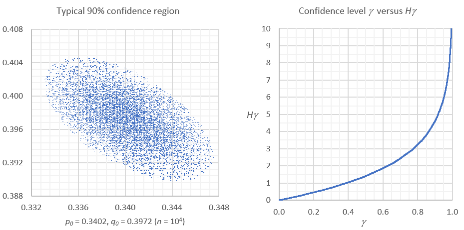
The dual confidence region is simply obtained by swapping the roles of (x, y) and (p, q) in Hn(x, y, p, q). It is thus defined as the set of (x, y) satisfying Hn(p, q, x, y) ≤ Hγ. Again, you choose Hγ to guarantee that the confidence level is γ. Also, (p, q) is replaced by (p0, q0). This is no longer the equation of an ellipse. In practice, both confidence regions are very similar. Also, Hγ is almost identical to Gγ. The interpretation is as follows. A point (x, y) is in the dual confidence region of (p0, q0) if and only if (p0, q0) is in the standard confidence region of (x, y). We use the same n and confidence level γ for both regions. You can use the same principle to define dual confidence intervals.
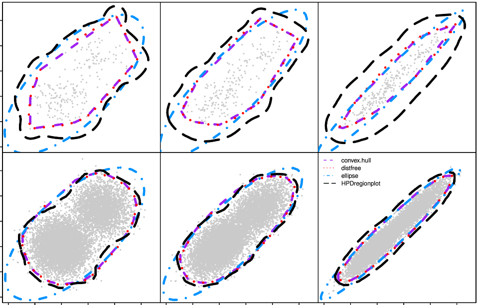
Figure 1 shows an example based on simulations.
Simulations
The simulations consist of generating N data sets, each with n observations. Use the joint Bernoulli model described in the first section, for the simulations. The purpose is to create data sets that have the same statistical behavior as your observations. In particular, use p0 and q0 in the bivariate Bernoulli model, for the simulations.
For each simulated data set, compute the proportions, standard deviations and correlations. They are denoted as x , y, σx, σy and ρx,y (one set of values per data set). Use the standard formulas from this article: for instance, σx = [x(1-x)]1/2. Also compute G(x, y) = Hn(x, y, p0, q0) and H(x, y) = Hn(p0, q0, x, y) for each data set. Put the results in a table with N rows and 7 columns. Proceed as follows.
- Standard confidence regions: sort the table by G(x, y).
- Dual confidence region: sort the table by H(x, y).
The first γN rows in your sorted table determines your confidence region of level γ. All the (x, y) in those rows belong to your confidence region. In the first γN rows, the last value of H(x, y) — if sorted by H(x, y) — is Hγ. Likewise, the last value of G(x, y) — if sorted by G(x, y) — is Gγ. See example in Figure 1, with N = 10,000 and n = 20,000. As N increases, your simulations yield regions closer and closer to the theoretical ones. The spreadsheet with these simulations is available on my GitHub repository, here.
The Original Problem
The original problem consisted of estimating the two parameters of a perturbed lattice point process. These stochastic processes have applications in sensor and cell network optimization. Rather than a direct estimation, I used proxy statistics p, q for the estimator. This method, called minimum contrast estimation, requires a one-to-one-mapping between the original parameter space, and the proxy space.
The point count statistic discussed earlier measures the number of points of this process that are in a specific interval Bk. I used n non-overlapping intervals B1, …, Bn, each one yielding one observation vector. The observation vectors are almost identically and independently distributed across the intervals. However, the first and second components of the vectors are negatively correlated. This explains the choice of the bivariate Bernoulli distribution for the model. The topic is discussed in details in my upcoming book, here.
About the Author

Vincent Granville is a pioneering data scientist and machine learning expert, founder of MLTechniques.com and co-founder of Data Science Central (acquired by TechTarget in 2020), former VC-funded executive, author and patent owner. Vincent’s past corporate experience includes Visa, Wells Fargo, eBay, NBC, Microsoft, CNET, InfoSpace. Vincent is also a former post-doc at Cambridge University, and the National Institute of Statistical Sciences (NISS).
Vincent published in Journal of Number Theory, Journal of the Royal Statistical Society (Series B), and IEEE Transactions on Pattern Analysis and Machine Intelligence. He is also the author of multiple books, available here. He lives in Washington state, and enjoys doing research on stochastic processes, dynamical systems, experimental math and probabilistic number theory.