
This post is a part of my forthcoming book on Mathematical foundations of Data Science.
In the previous blog, we saw how you could use basic high school maths to learn about the workings o…
In this post we extend that idea to learn about Gradient descent
We have seen that a regression problem can be modelled as a set of equations which we need to solve. In this section, we discuss the ways to solve these equations. Again, we start with ideas you learnt in school and we expand these to more complex techniques. In simple linear regression, we aim to find a relationship between two continuous variables. One variable is the independent variable and the other is the dependent variable (response variable). The relationship between these two variables is not deterministic but is statistical. In a deterministic relationship, one variable can be directly determined from the other. For example, conversion of temperature from Celsius to Fahrenheit is a deterministic process. In contrast, a statistical relationship does not have an exact solution – for example – the relationship between height and weight. In this case, we try to find the best fitting line which models the relationship. To find the best fitting line, we aim to reduce the total prediction error for all the points. Assuming a linear relation exists, the equation can be represented as y = mx + c for an input variable x and a response variable y. For such an equation, the values of m and c are chosen to represent the line which minimises the error. The error being defined as

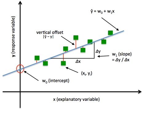
Image source and section adapted from sebastian raschka
This idea is depicted above.
More generally, for multiple linear regression, we have
y = m1x1 + m2x2 + m3x3
when expressed in the matrix form, this is represented as
y = X . m
Where X is the input data, m is a vector of coefficients and y is a vector of output variables for each row in X. To find the vector m, we need to solve the equation.
There are various ways to solve a set of linear equations
The closed form approach using the Matrix inverse
For smaller datasets, this equation can be solved by considering the matrix inverse. Typically, this was the way you learned to solve a set of linear equations in high school
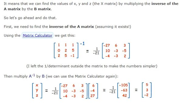
Source matrix inverse – maths is fun
This closed form solution is preferred for relatively smaller datasets where it is possible to compute the inverse of a matrix within a reasonable computational cost. The closed form solution based on computing the matrix inverse does not work large datasets or where the matrix inverse does not exist.
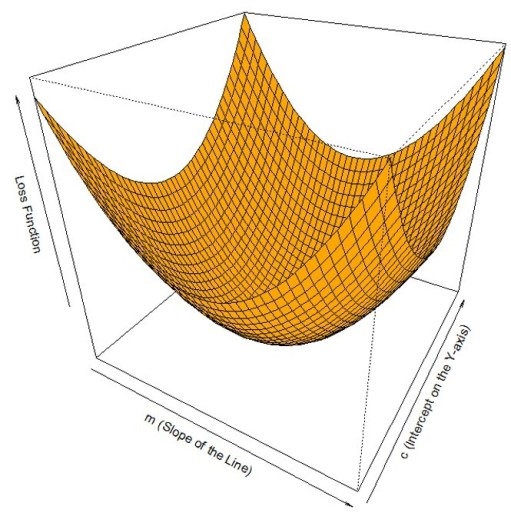
Instead of considering the matrix inverse, there is another way to solve a set of linear equations. Consider that the in the above diagram for the X and Y axes, the overall problem is to reduce the value of the loss function. In the above diagram, the cost function J(w), the sum of squared errors (SSE), can be written as:
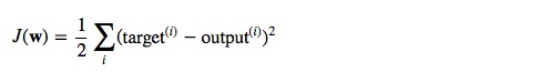
Hence, to solve these equations in a statistical manner (as opposed to deterministic), we need to find the minima of the above loss function. The minima of the loss function can be computed using an algorithm called Gradient Descent
The Gradient descent approach to solve linear equations
Typically, in two dimensions, the Gradient descent algorithm is depicted as a hiker (the weight coefficient) who wants to climb down a mountain (cost function) into a valley (representing the cost minimum), and each step is determined by the steepness of the slope (gradient). Considering a cost function with only a single weight coefficient, we can illustrate this concept as follows:
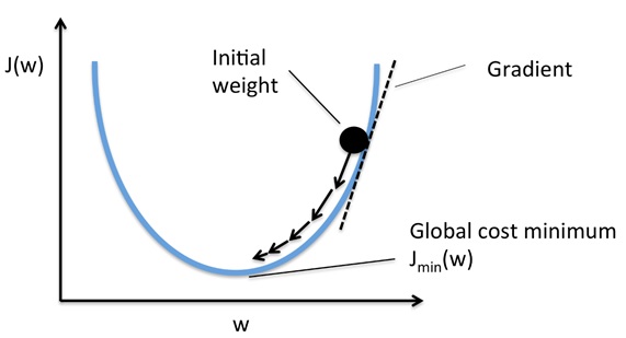
Using the Gradient Decent optimization algorithm, the weights are updated incrementally after each epoch (= pass over the training dataset). The magnitude and direction of the weight update is computed by taking a step in the opposite direction of the cost gradient. In three dimensions, solving this equation involves computing the minima of the loss function expressed in terms of slope and the intercept as below
http://ucanalytics.com/blogs/intuitive-machine-learning-gradient-de…
Use of Gradient descent in multi-layer perceptrons
You saw in the previous section, how the Gradient descent algorithm can be used to solve a linear equation. More typically, you are likely to encounter gradient descent to solve equations for multilayer perceptrons i.e. deep neural networks (where we have a set of non-linear equations). While the same principle applies, the context is different as we explain below
In a neural network, like the linear equation, we also have a loss function. Here, the loss function represents a performance metric which reflects how well the neural network generates values that are close to the desired values. The loss function is intuitively the difference between the desired output and the actual output. The goal of the neural network is to minimise the loss function for the whole network of neurons. Hence, the problem of solving equations represented by the neural network also becomes a problem of minimising the loss function. A combination of Gradient descent and backpropagation algorithms are used to train a neural network i.e. to minimise the total loss function
The overall steps are
- In forward propagate, the data flows through the network to get the outputs
- The loss function is used to calculate the total error
- Then, we use backpropagation algorithm to calculate the gradient of the loss function with respect to each weight and bias
- Finally, we use Gradient descent to update the weights and biases at each layer
- Repeat above steps to minimize the total error of the neural network.
Hence, in a single sentence we are essentially propagating the total error backward through the connections in the network layer by layer, calculate the contribution (gradient) of each weight and bias to the total error in every layer, then use gradient descent algorithm to optimize the weights and biases, and eventually minimize the total error of the neural network.
Explaining the forward pass and the backward pass
In a neural network, the forward pass is a set of operations which transform network input into the output space. During the inference stage neural network relies solely on the forward pass. For the backward pass, in order to start calculating error gradients, first, we have to calculate the error (i.e. the overall loss). We can view the whole neural network as a composite function (a function comprising of other functions). Using the Chain Rule, we can find the derivative of a composite function. This gives us the individual gradients. In other words, we can use the Chain rule to apportion the total error to the various layers of the neural network. This represents the gradient that will be minimised using Gradient Descent.
A recap of the Chain Rule and Partial Derivatives
We can thus see the process of training a neural network as a combination of Back propagation and Gradient descent. These two algorithms can be explained by understanding the Chain Rule and Partial Derivatives.
The Chain Rule
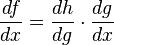
The chain rule is a formula for calculating the derivatives of composite functions. Composite functions are functions composed of functions inside other function(s). Given a composite function f(x) = h(g(x)), the derivative of f(x) is given by the chain rule as
You can also extend this idea to more than two functions. For example, for a function f(x) comprising of three functions A, B and C – we have
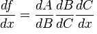
f(x) = A(B(C(x)))
The chain rule tells us that the derivative of this function equals:
Gradient Descent and Partial Derivatives
As we have seen before, Gradient descent is an iterative optimization algorithm which is used to find the local minima or global minima of a function. The algorithm works using the following steps
- We start from a point on the graph of a function
- We find the direction from that point, in which the function decreases fastest
- We travel (down along the path) indicated by this direction in a small step to arrive at a new point
The slope of a line at a specific point is represented by its derivative. However, since we are concerned with two or more variables (weights and biases), we need to consider the partial derivatives. Hence, a gradient is a vector that stores the partial derivatives of multivariable functions. It helps us calculate the slope at a specific point on a curve for functions with multiple independent variables. We need to consider partial derivatives because for complex(multivariable) functions, we need to determine the impact of each individual variable on the overall derivative. Consider a function of two variables x and z. If we change x, but hold all other variables constant, we get one partial derivative. If we change z, but hold x constant, we get another partial derivative. The combination represents the full derivative of the multivariable function.
Conclusion
In this post, you understood the application of Gradient descent both in neural networks but also back to linear equations
Please follow me on Linkedin – Ajit Jaokar if you wish to stay updated about the book
References