
This post is a part of my forthcoming book on Mathematical foundations of Data Science.
In this post, we use the Perceptron algorithm to bridge the gap between high school maths and deep learning. Welcome comments
Background
As part of my role as course director of the Artificial Intelligence: Cloud and Edge Computing at the University…, I see more students who are familiar with programming than with mathematics.
They have last learnt maths years ago at University. And then, suddenly they find that they encounter matrices, linear algebra etc when they start learning Data Science.
Ideas they thought they would not face again after college! Worse still, in many cases, they do not know where precisely these concepts apply to data science.
If you consider the maths foundations needed to learn data science, you could divide them into four key areas
- Linear Algebra
- Probability Theory and Statistics
- Multivariate Calculus
- Optimization
All of these are taught (at least partially) in high schools (14 to 17 years of age).
In this book, we start with these ideas and co-relate them to data science and AI.
Understanding Linear Regression
Let’s start with Linear Regression
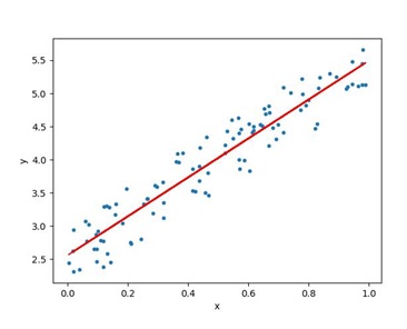
A linear relationship means that you can represent the relationship between two sets of variables with a straight line. Many phenomena can be represented by a linear relationship. We can represent this relationship in the form of a linear equation in the form:
y = mx + b
Where:
“m” is the slope of the line,
“x” is any point (an input or x-value) on the line,
and “b” is where the line crosses the y-axis.
The relationship can be represented as below:
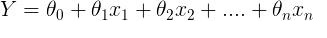
If we expand this equation more generally to n variables we get
Let us now switch tools to a new type of model i.e. from Linear regression to Perceptron learning. We show how this new model and linear regression are related. In addition, perceptron learning can be expanded to multilayer perceptrons i.e. Deep Learning algorithms.
Perceptron learning
A perceptron can be seen as an ‘artificial neuron’ i.e. a simplified version of a biological neuron. In the simplest case, a perceptron is represented as below. A perceptron takes several inputs, x1,x2,…x1,x2,…, and produces a single binary output:
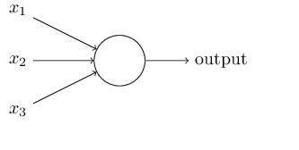
Figure: Perceptron
Expanding the above, in the example shown below we now consider weighted inputs. The perceptron has three inputs, x1 ,x2, x3 and weights, w1,w2,…w1,w2,…, are real numbers expressing the importance of the respective inputs to the output. The perceptron’s output, 0 or 1, is determined by whether the weighted sum ∑jwjxj is less than or greater than some threshold value. We can think of the perceptron as a device that makes decisions by weighing up evidence. This idea is similar to the multiple linear equation we have seen before. This idea can be represented as a function as shown below.
Figure: A generic representation of a perceptron
which is indeed similar to the equation of multiple linear regression we have seen before
The Perceptron – more than a footnote in history
As an algorithm, perceptrons have an interesting history. Perceptrons started off being implemented in hardware. The Mark I Perceptron machine was the first implementation of the perceptron algorithm. The perceptron algorithm was invented in 1957 at the Cornell Aeronautical Laboratory by Frank Rosenblatt. The perceptron was intended to be a machine, rather than a program. This machine was designed for image recognition: it had an array of 400 photocells, randomly connected to the “neurons”. Weights were encoded in potentiometers, and weight updates during learning were performed by electric motors. There was misplaced optimism about perceptrons. In a 1958 press conference organized by the US Navy, Rosenblatt made statements about the perceptron that caused a controversy among the fledgeling AI community; based on Rosenblatt’s statements, The New York Times reported the perceptron to be “the embryo of an electronic computer that [the Navy] expects will be able to walk, talk, see, write, reproduce itself and be conscious of its existence.”
Although the perceptron initially seemed promising, it was quickly proved that perceptrons could not be trained to recognise many classes of patterns. This misplaced optimism caused the field of neural network research to stagnate for many years before it was recognised that a feedforward neural network with two or more layers (also called a multilayer perceptron) had far greater processing power than perceptrons with one layer (i.e. single layer perceptron). Single layer perceptrons are only capable of learning linearly separable patterns.
Below is an example of a learning algorithm for a (single-layer) perceptron. A diagram showing a perceptron updating its linear boundary as more training examples are added.
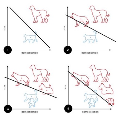
Figure: Perceptron classification
Above description of Perceptrons and Image – adapted from Wikipedia
Thus, while the perceptron is of historical significance, it is a functioning algorithm i.e. a linear classifier. A linear classifier is interesting, but it is not compelling enough as per the initial promises and potential.
However, for us, a Perceptron is more than a footnote in history. It is a way to bridge your basic high school knowledge with Deep Learning
Overcoming the limitations of Perceptron Learning using non-linear activation functions
One step towards overcoming the limitations of Perceptrons of being only a linear classifier is to consider non-linear activation functions. In the figure above (Figure: A generic representation of a perceptron) – the function f represents the activation function. In case of a perceptron, the activation function is only a step function. The step function output represents the output of the perceptron. The input of the step function is the weighted inputs. We discuss activation functions in more detail below. But for now, it is important to realise that the activation function for the perceptron is a step function.
In 1969, a famous book entitled Perceptrons by Marvin Minsky and Seymour Papert showed that it was impossible for perceptrons to learn an XOR function. However, this limitation does not apply if we use a non-linear activation function (instead of a step function) for a perceptron. In fact, by using non-linear activation functions, we can model many more complex functions than the XOR (even with just the single layer). This idea can be extended if we add more hidden layers – creating the multilayer perceptron.
The working of activation function can be understood by finding the mapped value of y on the curve for given x. sigmoid, tanH, ReLU are examples of activation functions. For example, the sigmoid activation function maps a range of values between 0 and 1. This means, for values of x between minus infinity to plus infinity, the value of y will be mapped to between 0 and 1 by the sigmoid function. For each node, sigmoid activation gives the output as sigmoid (dot(input, weights) ) + b – where the input to the function represents the dot product of the x values and weights at each node. The matrix b represents the matrix of biases. Similarly, the tanh function represents an output that lies between -1 and +1. Activation functions need to be differentiable because the derivate of the function represents the direction of change when the steps are updated.
So, to recap:
- The perceptron is a simplified model of a biological neuron.
- The perceptron is an algorithm for learning a binary classifier: a function that maps its input to an output value (a single binary value).
- A perceptron is an artificial neuron using the step function as the activation function ([1]). The perceptron algorithm is also termed the single-layer perceptron, to distinguish it from a multilayer perceptron.
- While the Perceptron algorithm is of historical significance, it provides us with a way to bridge the gap between Linear Regression and Multi-Layer Perceptrons i.e. Deep Learning.
Multi-layer perceptrons
We now come to the idea of the Multi-layer perceptron(MLP). Multilayer perceptrons overcome the limitations of the perceptron algorithm discussed in the previous section by three means:
- By using non-linear activation functions and
- By using multiple layers of perceptrons (instead of a single perceptron).
- Using a different method of training i.e. the MLP needs a combination of backpropagation and gradient descent for training.
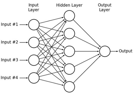
Figure: multilayer perceptron
Thus, MLPs can be seen as a complex network of perceptrons (with non-linear activation functions) and they can make subtle and complex decisions based on weighing up evidence hierarchically.
To conclude
In this post, we used the Perceptron to bridge the gap between Linear Regression (taught in schools) with Multi-layer Perceptrons (Deep Learning). Please follow me on Linkedin – Ajit Jaokar if you wish to stay updated about the book