
Brian Huge and I just posted a working paper following six months of research and development on function approximation by artificial intelligence (AI) in Danske Bank. One major finding was that training machine learning (ML) models for regression (i.e. prediction of values, not classes) may be massively improved when the gradients of training labels wrt training inputs are available. Given those differential labels, we can write simple, yet unreasonably effective training algorithms, capable of learning accurate function approximations with remarkable speed and accuracy from small datasets, in a stable manner, without the need of additional regularization or optimization of hyperparameters, e.g. by cross-validation.
In this post, we briefly summarize these algorithms under the name differential machine learning, highlighting the main intuitions and benefits and commenting TensorFlow implementation code. All the details are found in the working paper, the online appendices and the Colab notebooks.
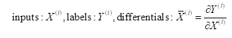
In the context of financial Derivatives pricing approximation, training sets are simulated with Monte-Carlo models. Each training example is simulated on one Monte-Carlo path, where the label is the final payoff of a transaction and the input is the initial state vector of the market. Differential labels are the pathwise gradients of the payoff wrt to the state and efficiently computed with Automatic Adjoint Differentiation (AAD). For this reason, differential machine learning is particularly effective in finance, although it is also applicable in all other situations where high-quality first-order derivatives wrt training inputs are available.
Models are trained on augmented datasets of not only inputs and labels but also differentials:
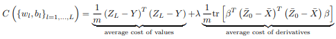
The value and derivative labels are given. We compute predicted values by inference, as customary, and predicted derivatives by backpropagation. Although the methodology applies to architectures of arbitrary complexity, we discuss it here in the context of vanilla feedforward networks in the interest of simplicity.
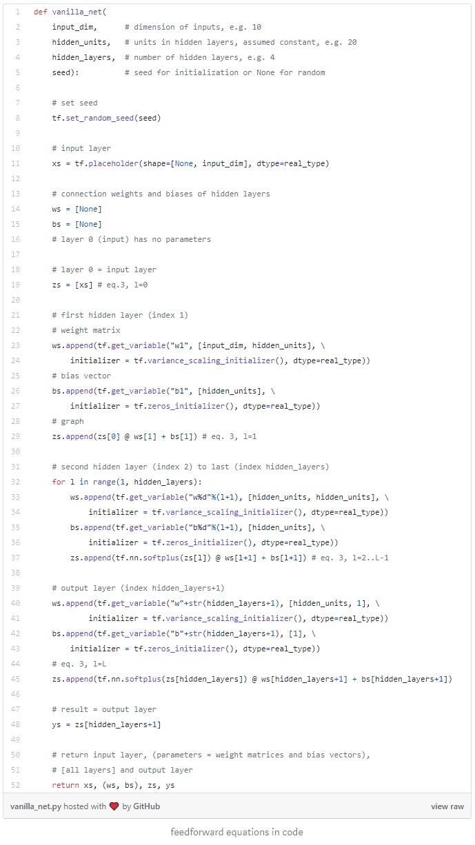
Recall vanilla feedforward equations:
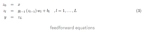
where the notations are standard and specified in the paper (index 3 is for consistency with the paper).
All the code in this post is extracted from the demonstration notebook, which also includes comments and practical implementation details.

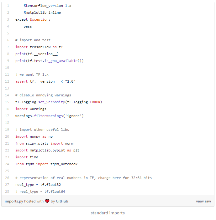
Below is a TensorFlow (1.x) implementation of the feedforward equations. We chose to write matrix operations explicitly in place of high-level Keras layers to highlight equations in code. We chose soft plus activation. ELU is another alternative. For reasons explained in the paper, activation must be continuously differentiable, ruling out e.g. RELU and SELU.
Derivatives of output wrt inputs are predicted with backpropagation. Recall backpropagation equations are derived as adjoints of the feedforward equations, or see our tutorial for a refresh:
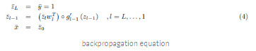
Or in code, recalling that the derivative of softplus is sigmoid:
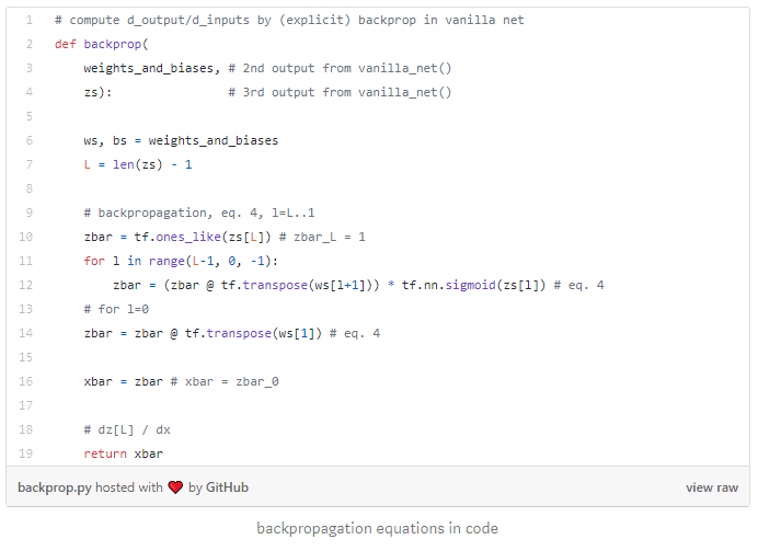
Once again, we wrote backpropagation equations explicitly in place of a call to tf.gradients(). We chose to do it this way, first, to highlight equations in code again, and also, to avoid nesting layers of backpropagation during training, as seen next. For the avoidance of doubt, replacing this code by one call to tf.gradients() works too.
Next, we combine feedforward and backpropagation in one network, which we call twin network, a neural network of twice the depth, capable of simultaneously predicting values and derivatives for twice computation cost:
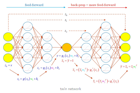
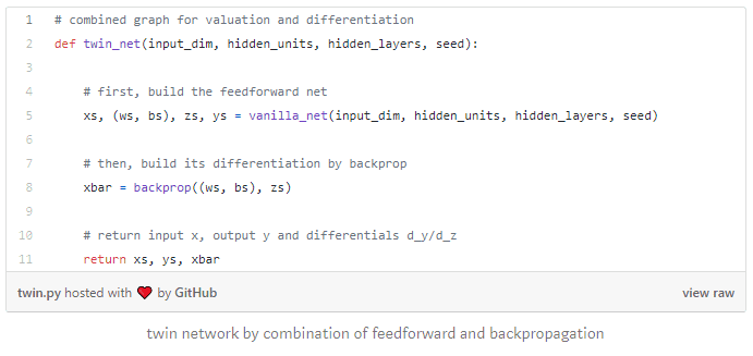
The twin network is beneficial in two ways. After training, it efficiently predicts values and derivatives given inputs in applications where derivatives predictions are desirable. In finance, for example, they are sensitivities of prices to market state variables, also called Greeks (because traders give them Greek letters), and also correspond to hedge ratios.
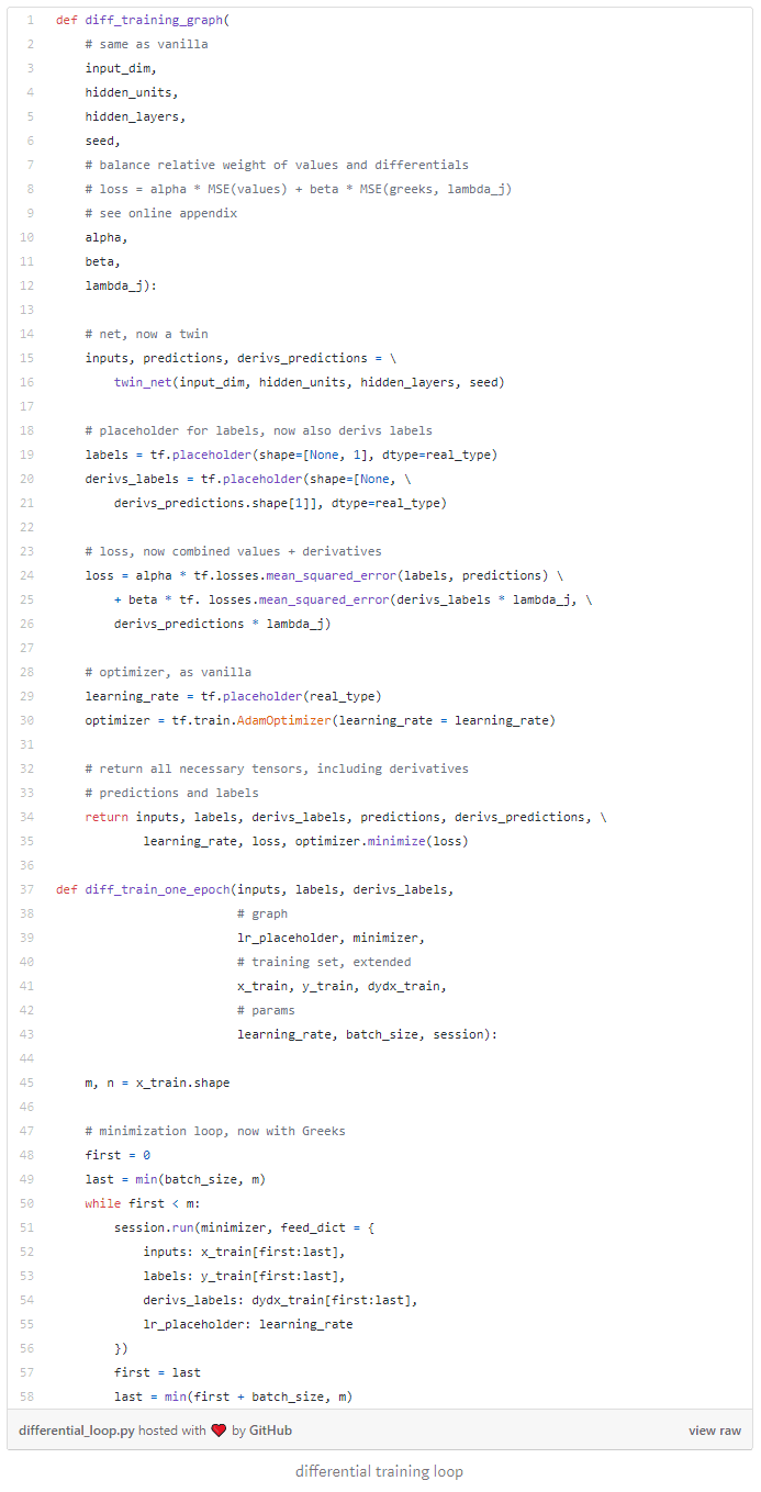
The twin network is also a fundamental construct for differential training. The combined cost function is computed by inference through the twin network, predicting values and derivatives. The gradients of the cost function are computed by backpropagation through the twin network, including the backpropagation part, silently conducted by TensorFlow as part of its optimization loop. Recall the standard training loop for neural networks:
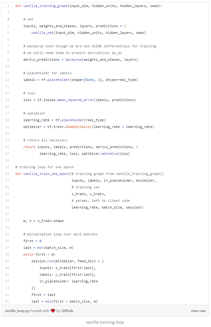
TensorFlow differentiates the twin network seamlessly behind the scenes for the needs of optimization. It doesn’t matter that part of the network is itself a backpropagation. This is just another sequence of matrix operations, which TensorFlow differentiates without difficulty.
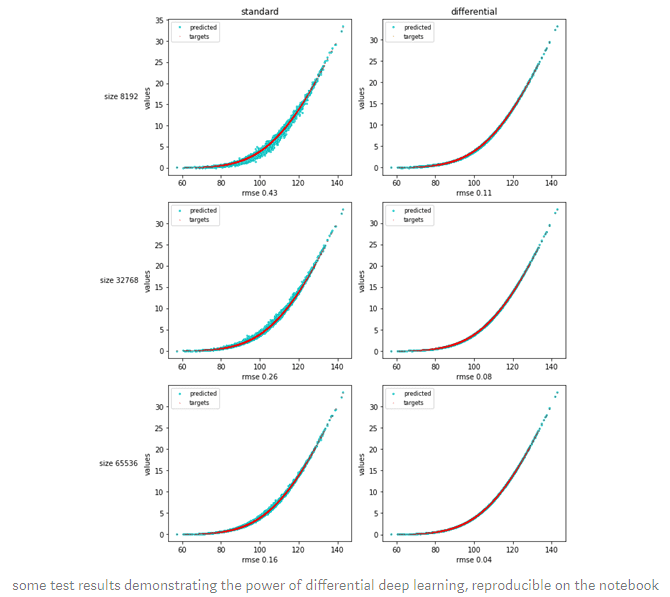
The rest of the notebook deals with standard data preparation, training and testing and the application to a couple of textbook datasets in finance: European calls in Black & Scholes, and basket options in correlated Bachelier. The results demonstrate the unreasonable effectiveness of differential deep learning.
In the online appendices, we explored applications of differential machine learning to other kinds of ML models, like basis function regression and principal component analysis (PCA), with equally remarkable results.
Differential training imposes a penalty on incorrect derivatives in the same way that conventional regularization like ridge/Tikhonov favours small weights. Contrarily to conventional regularization, differential ML effectively mitigates overfitting without introducing bias. Hence, there is no bias-variance tradeoff or necessity to tweak hyperparameters by cross-validation. It just works.
Differential machine learning is more similar to data augmentation, which in turn may be seen as a better form of regularization. Data augmentation is consistently applied e.g. in computer vision with documented success. The idea is to produce multiple labelled images from a single one, e.g. by cropping, zooming, rotation or recolouring. In addition to extending the training set for negligible cost, data augmentation teaches the ML model important invariances. Similarly, derivatives labels, not only increase the amount of information in the training set for a very small cost (as long as they are computed with AAD) but also teach ML models the shape of pricing functions.
Working paper: https://arxiv.org/abs/2005.02347
Github repo: github.com/differential-machine-learning
Colab Notebook: https://colab.research.google.com/github/differential-machine-learn…
Originally posted here