Introduction

In this post, I explain the maths of Deep Learning in a simplified manner. To keep the explanation simple, we cover the workings of the MLP mode (Multilayer Perceptron). I have drawn upon a number of references – which are indicated in the post in the relevant sections.

Deep Learning models are playing a significant role in many domains. In the simplest case, deep learning involves stacking multiple neural network layers to address a problem (typically Classification). Deep neural networks can handle a large number of features and can perform automatic feature selection. Prior to Deep neural networks, algorithms like SVM performed linear classification (and non-linear classification using the Kernel trick). But SVM still needs explicit feature selection and feature transformation techniques. In 2012, Geoffrey Hinton used generalized backpropagation algorithm for training a multi-layer neural network. With this development, the field of deep learning – as we know it today – was born. Other factors also benefited Deep Learning – for example the availability of Data and better processing power (GPUs) etc

The fundamental unit of a neural net is a single neuron which was loosely modelled after the neurons in a biological brain. For the simplest case (MLP – Multilayer perceptron), each neuron in a given layer (i.e., layer 1) will be connected to neurons in the next layer (i.e., layer 2). The connections between neurons mimic the synapses in the biological brain. A neuron will only fire i.e. send the output signal if the weighted summation of its input signals transformed by an activation function passes a threshold. The activation function is non-linear

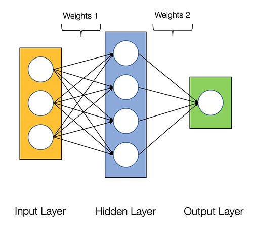
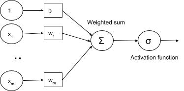
Image source: O Reilly

Understanding the significance of non-linearity

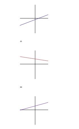
Before we proceed, we need to appreciate the significance of non-linearlity. Why do we need to use non-linear activation functions? What is the significance and benefit of non-linear functions? In a nutshell, without a non-linear activation function, the neural network is merely calculating linear combinations of values i.e. the network is combining the signals but is not creating a new signal / function. For example, the linear combination of two lines is another line. As we see below.

However, with a non-linear activation function like ReLU, the linear combination is a new type of function. We can construct entirely different (nonlinear) models in this way. So, introducing nonlinearity extends the kinds of functions that we can represent with our neural network.

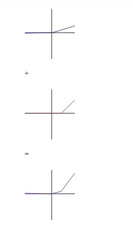
Reference and image Quora Why does deep learning architectures only use the non-linear …

Training a Neural Network

Training steps

The loss function is a performance metric which reflects how well the neural network generates values that are close to the desired values. The loss function is intuitively the difference between the desired output and the actual output. The goal of machine learning is to minimise the loss function. Hence, the problem of machine learning becomes a problem of minimising the loss function.

A combination of Gradient descent and backpropagation algorithms are used to train a neural network i.e. to minimise the total loss function

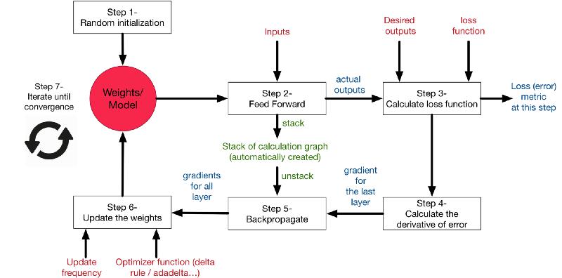
The overall steps are

Forward propagate the data points through the network get the outputs
Use loss function to calculate the total error
Use backpropagation algorithm to calculate the gradient of the loss function with respect to each weight and bias
Use Gradient descent to update the weights and biases at each layer
Repeat above steps to minimize the total error.

Hence, in a single sentence we are essentially propagating the total error backward through the connections in the network layer by layer, calculate the contribution (gradient) of each weight and bias to the total error in every layer, then use gradient descent algorithm to optimize the weights and biases, and eventually minimize the total error of the neural network.

reference Ken Chen on linkedin

Explaining the forward pass and the backward pass

Forward Pass

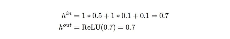
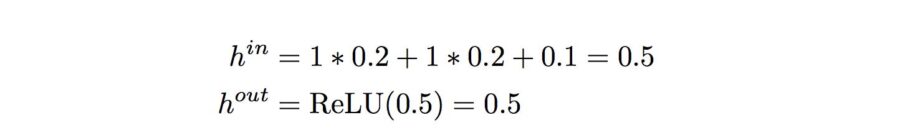
Forward pass is basically a set of operations which transform network input into the output space. During the inference stage neural network relies solely on the forward pass. Let’s consider a simple neural network with 2-hidden layers. Here we assume that each neuron, except the neurons in the last layers, uses ReLU activation function (the last layer uses softmax).

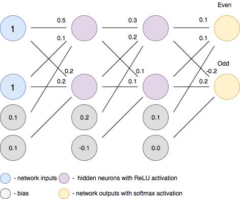
neuron 1 (top):

neuron 2 (bottom):

Rewriting this into a matrix form we will get:

Backward Pass

In order to start calculating error gradients, first, we have to calculate the error (i.e. the overall loss). We can view the whole neural network as a composite function (a function comprising of other functions). Using the Chain Rule, we can find the derivative of a composite function. This gives us the individual gradients. In other words, we can use the Chain rule to apportion the total error to the various layers of the neural network. This represents the gradient that will be minimised using Gradient Descent.

Reference and image source: under the hood of neural networks part 1 fully connected

A recap of the Chain Rule and Partial Derivatives

We can thus see the process of training a neural network as a combination of Back propagation and Gradient descent. These two algorithms can be explained by understanding the Chain Rule and Partial Derivatives.

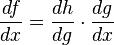
The Chain Rule

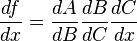
The chain rule is a formula for calculating the derivatives of composite functions. Composite functions are functions composed of functions inside other function(s). Given a composite function f(x) = h(g(x)), the derivative of f(x) is given by the chain rule as

You can also extend this idea to more than two functions. For example, for a function f(x) comprising of three functions A, B and C – we have

f(x) = A(B(C(x)))

The chain rule tells us that the derivative of this function equals:

Gradient Descent and Partial Derivatives

Gradient descent is an iterative optimization algorithm which is used to find the local minima or global minima of a function. The algorithm works using the following steps

We start from a point on the graph of a function
We find the direction from that point, in which the function decreases fastest
We travel (down along the path) indicated by this direction in a small step to arrive at a new point

The slope of a line at a specific point is represented by its derivative. However, since we are concerned with two or more variables (weights and biases), we need to consider the partial derivatives. Hence, a gradient is a vector that stores the partial derivatives of multivariable functions. It helps us calculate the slope at a specific point on a curve for functions with multiple independent variables. We need to consider partial derivatives because for complex(multivariable) functions, we need to determine the impact of each individual variable on the overall derivative. Consider a function of two variables x and z. If we change x, but hold all other variables constant, we get one partial derivative. If we change z, but hold x constant, we get another partial derivative. The combination represents the full derivative of the multivariable function.

Thus, the entire neural network training can be seen as a combination of the chain rule and partial derivatives

Reference and image source – neural networks and backpropagation explained in a simple way

Big Picture

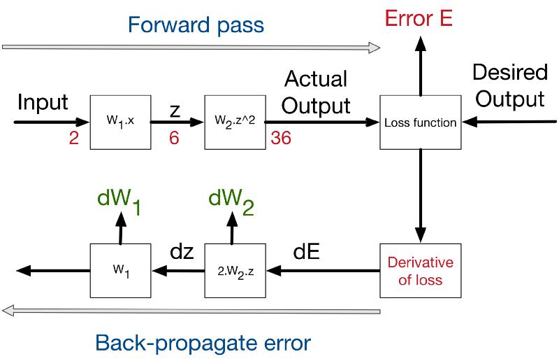
To recap, considering the big picture – we have the starting point of errors, which is the loss function. This figure shows the process of backpropagating errors following this schemas:
Input -> Forward calls -> Loss function -> derivative -> backpropagation of errors. At each stage we get the deltas on the weights of this stage. For the figure below, W1 = 3 and w2 = 1