Numerical Modality

The mode is one of the basic statistics which is defined as the most common value over an array. When the values of the array are categorical, the mode is easy to detect by selecting the one with the most occurrence. The problem of identifying the modes on a numerical array is harder since the values can be continuous and therefore count the occurrences by value is not enough, so the distribution of these values must be checked in order to identify the most probable values. However, numerical arrays can be multi-modal which reduces the problem to finding local maxima on the distribution instead of the global maximum where only one mode is present.

Detecting local maxima with histograms

Finding histograms is one of the easiest ways to find the distribution of a numerical array. By looking at the distribution it might be clear where the modes are.

To show that, an array of values is generated by simulated values from various normal distributions, as shown in the code below.

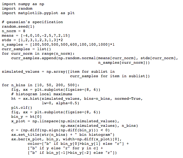
Here are four histograms of the previous simulated values changing the number of bins. As can be seen, the local maxima are colored blue, and the number of local maxima changes depending on the number of bins in the histogram.

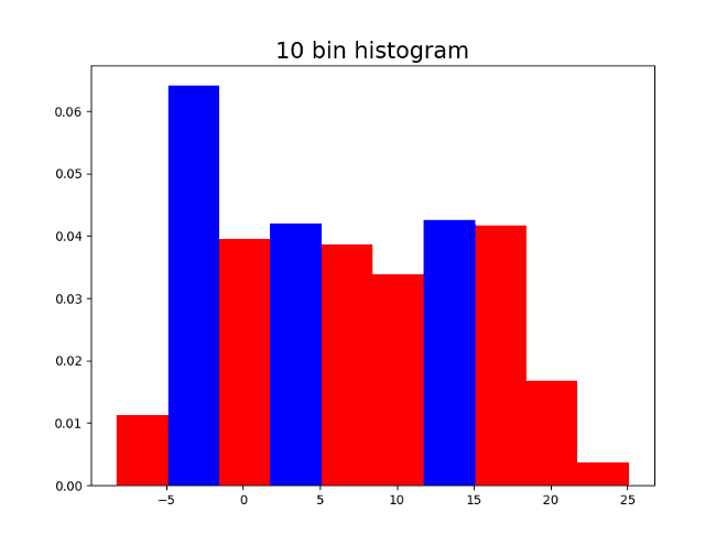
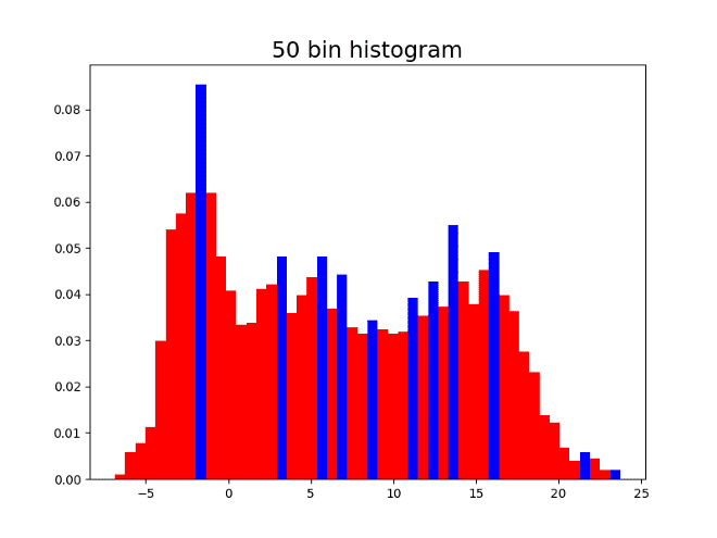
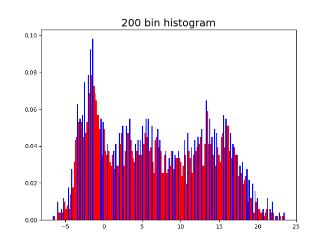
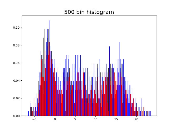
Having 10 bins might seem reasonable since 3 might be the correct number of modes. On the other hand, having the 500 bins shows the shape of the distribution but does not allow to identify the modes since there are many local maxima. It is convenient to capture a good approximation of the number of modes in a systematic way, with no need of the human eye intervention.

Dirichlet Process Mixture Model

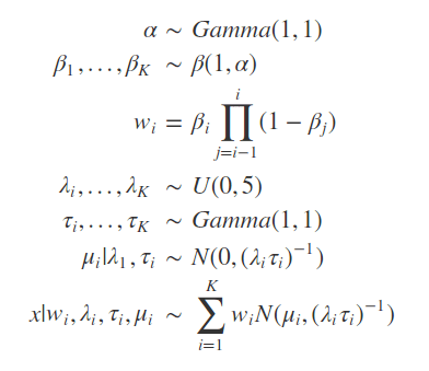
Mixture models are generated by the aggregation of sub-models, each of them weighted by their own parameter. For this example the weights are simulated by a Dirichlet Process and sum to one, this weights can be simulated by a stick breaking process. Each of the models that add up is Gaussian with their respective parameters.

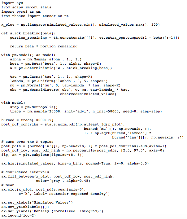
The number of sub-models is denoted by K and set to 50. As seen below, the model has high complexity and the use of probabilistic programming methods is needed to make it’s estimation feasible.

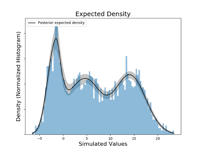
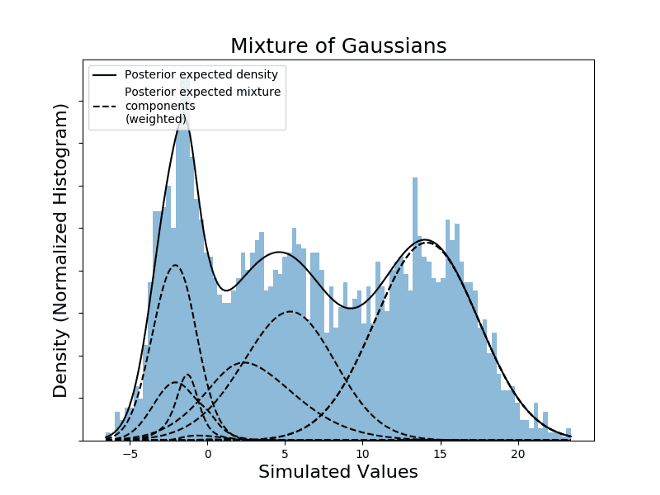
By checking the local maxima on the expected density, it is possible to check that the values in the domain that results on maxima are: -1.57, 4.59, 14.07. The estimation was done without knowing the exact number of modes, by setting K large enough to host all the possible Gaussian distributions that together form the PDF (Probability Density Function) of the values.

(This blog post originally appeared here)