
In this series, we discuss a technique to find either the minima or the roots of a chaotic, unsmooth, or discrete function. A root-finding technique that works well for continuous, differentiable functions is successfully adapted and applied to piece-wise constant functions with an infinite number of discontinuities. It even works if the function has no root: it will then find minima instead. In order to work, some constraints must be put on the parameters used in the algorithm, while avoiding over-fitting at the same time. This would also be true true anyway for the smooth, continuous, differentiable case. It does not work in the classical sense where an iterative algorithm converges to a solution. Here the iterative algorithm always diverges, yet it has a clear stopping rule that tells us when we are very close to a solution, and what to do to find the exact solution. This is the originality of the method, and why I call it new. Our technique, like many machine learning techniques, can generate false positives or false negatives, and one aspect of our methodology is to minimize this problem.
Applications are discussed, as well as full implementation with results, for a real-life, challenging case, and on simulated data. This first article in this series is a detailed introduction. Interestingly, we also show an example where a continuous, differentiable function, with a very large number of wild oscillations, benefit from being transformed into a non-continuous, non-differentiable function and then use our non-standard technique to find roots (or minima) as the standard technique fails. For the moment, we limit ourselves to the one-dimensional case.
1. Example of problem
In the following, a = 7919 x 3083 is a constant, and b is the variable. We try to find the two roots b = 7919 and b = 3083 (both prime numbers) of the function f(b) = 2 – cos(2Ïb) – cos(2Ïa/b). We will just look between b = 2000 and b = 4000, to find the root b = 3083. This function is plotted below, between b = 2900 and b = 3200. The X-axis represents b, the Y-axis represents f(b).
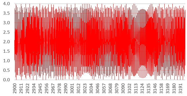
Despite the appearances, this function is well behaved, smooth, continuous and differentiable everywhere between b = 2000 and b = 4000. Yet, it is no surprise that classical root-finding or minimum-finding algorithms such as Newton-Raphson (see here) fail, or require a very large number of iterations to converge, or require to start very close to the unknown root, and are thus of no practical value.
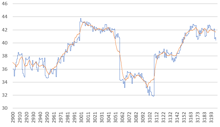
In this example, clearly f(b) = 0 in the interval 2000 < b < 4000 (and this is also the minimum possible value) if and only if b divides a. In other to solve this problem, we transformed f into a new function g, which despite being unsmooth, lead to a much faster algorithm. The new function g, as well as its smoothed version h, are pictured below (g is in blue, h is in red). In this case, our method solves the factoring problem (factoring the number a) in relatively few iterations, potentially much faster than sequentially identifying and trying all the 138 prime divisors of a that are between 2000 and 3083.
However, this is not by far the best factoring algorithm as it was not designed specifically for that purpose, but rather for general purpose. In a subsequent article part of this series, we apply the methodology to data that behaves somehow like in this example, but with random numbers: in that case, it is impossible to “guess” what the roots are, yet the algorithm is just as efficient.
2. Fundamentals of our new algorithm
This section outlines the main features of the algorithm. First, you want to magnify the effect of the root. In the first figure, roots (or minima) are invisible to the naked eye, or at least undistinguishable from many other values that are very close to zero. To achieve this goal (assuming f is positive everywhere) replace a suitably discretized version of f(x) by g(x) = log(ε + λf(x)), with ε > 0 close to zero. Then, in order to enlarge the width of the “hole” created around a root (in this case around b = 3083), you use some kind of moving average, possibly followed by a shift on the Y-axis.
The algorithm then proceeds as fixed-point iterations: bn+1 = bn + μ g(bn). Here we started with b0 = 2000. Rescaling is optional, if you want to keep the iterates bounded. One that does this trick here, is bn+1 = bn + μ g(bn) / SQRT(bn). Assuming the iterations approach the root (or minima) from the right direction, once it hits the “hole”, the algorithm emits a signal, but then continue without ever ending, without ever converging. You stop when you see the signal, or after a fixed number of iterations if no signal ever shows up. In the latter case, you just missed the root (the equivalent of a false negative).
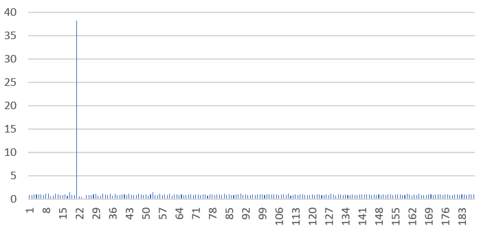
The signal is measured as the ratio (bn – bn-1) / (bn+1 – bn) which dramatically spikes just after entering the hole, depending on the parameters. In some cases, the signal may be weaker (or absent or multiple signals), and can result in false positives. Even if there is no root but a minimum instead, as in the above figure, the signal may still be present. Below is a picture featuring the signal, occurring at iteration n = 22: it signals that b21 = 3085.834 is in close vicinity of the root b = 3082. The X-axis represents the iteration number in the fixed point algorithm. How close to a root you end up is determined by the size of the window used for the moving average.
The closest to my methodology, in the literature, is probably the discrete fixed point algorithm, see here.
3. Details
All the details will be provided in the next articles in this series. To not miss them, you can subscribe to our newsletter, here. We will discuss the following:
- Source code and potential applications (e.g. Brownian bridges)
- How to smooth chaotic curves, and visualization issues (see our red curve in the second figure – we will discuss how it was created)
- How to optimize the parameters in our method without overfitting
- How to improve our algorithm
- How we used only local optimization without storing a large table of f or g values, yet finding a global minimum or a root (this is very useful if your target interval to find a minimum or root is very large, or if each call to f or g is very time consuming)
- A discussion on how to generalize the modulus function to non-integer numbers, and investigate the properties of modulus functions for real numbers, not just integers.
About the author: Vincent Granville is a machine learning scientist, author and publisher. He was the co-founder of Data Science Central (acquired by TechTarget) and most recently, founder of Machine Learning Recipes.
nn