
This problem appeared as a project in the edX course ColumbiaX: CSMM.101x Artificial Intelligence (AI). In this assignment an agent will be implemented to solve the 8-puzzle game (and the game generalized to an n × n array).
The following description of the problem is taken from the course:
I. Introduction
An instance of the n-puzzle game consists of a board holding n^2-1 distinct movable tiles, plus an empty space. The tiles are numbers from the set 1,..,n^2-1. For any such board, the empty space may be legally swapped with any tile horizontally or vertically adjacent to it. In this assignment, the blank space is going to be represented with the number 0. Given an initial state of the board, the combinatorial search problem is to find a sequence of moves that transitions this state to the goal state; that is, the configuration with all tiles arranged in ascending order 0,1,… ,n^2−1. The search space is the set of all possible states reachable from the initial state. The blank space may be swapped with a component in one of the four directions {‘Up’, ‘Down’, ‘Left’, ‘Right’}, one move at a time. The cost of moving from one configuration of the board to another is the same and equal to one. Thus, the total cost of path is equal to the number of moves made from the initial state to the goal state.
II. Algorithm Review
The searches begin by visiting the root node of the search tree, given by the initial state. Among other book-keeping details, three major things happen in sequence in order to visit a node:
- First, we remove a node from the frontier set.
- Second, we check the state against the goal state to determine if a solution has been found.
- Finally, if the result of the check is negative, we then expand the node. To expand a given node, we generate successor nodes adjacent to the current node, and add them to the frontier set. Note that if these successor nodes are already in the frontier, or have already been visited, then they should not be added to the frontier again.
This describes the life-cycle of a visit, and is the basic order of operations for search agents in this assignment—(1) remove, (2) check, and (3) expand. In this assignment, we will implement algorithms as described here.
III. What The Program Need to Output
Example: Breadth-First Search
Suppose the program is executed for breadth-first search starting from the initial state 1,2,5,3,4,0,6,7,8 as follows:
The output file should contain exactly the following lines:
path_to_goal: [‘Up’, ‘Left’, ‘Left’]
cost_of_path: 3
nodes_expanded: 10
fringe_size: 11
max_fringe_size: 12
search_depth: 3
max_search_depth: 4
running_time: 0.00188088
max_ram_usage: 0.07812500
The following algorithms are going to be implemented and taken from the lecture slides from the same course.
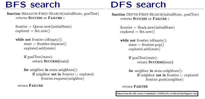
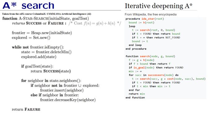
Outputs
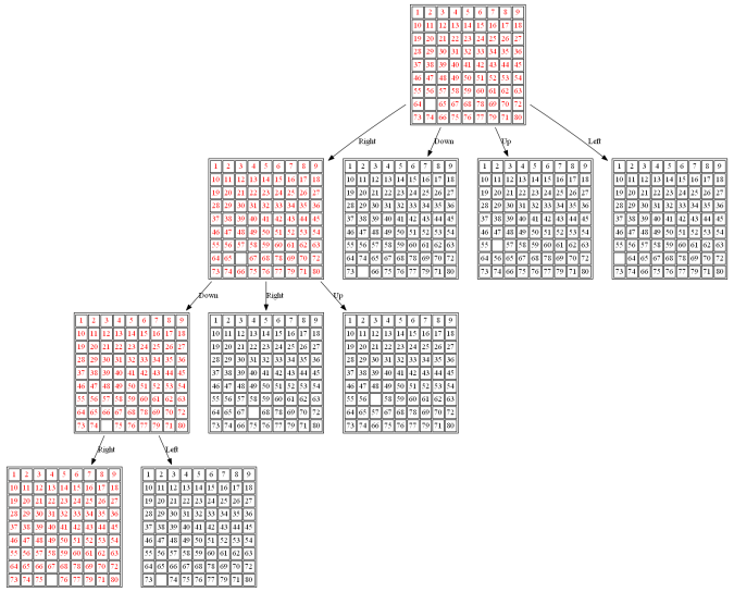
The following figures and animations show how the 8-puzzle was solved starting from different initial states with different algorithms. For A* and ID-A* search we are going to use Manhattan heuristic, which is an admissible heuristic for this problem. Also, the figures display the search paths from starting state to the goal node (the states with red text denote the path chosen). Let’s start with a very simple example. As can be seen, with this simple example all the algorithms find the same path to the goal node from the initial state.
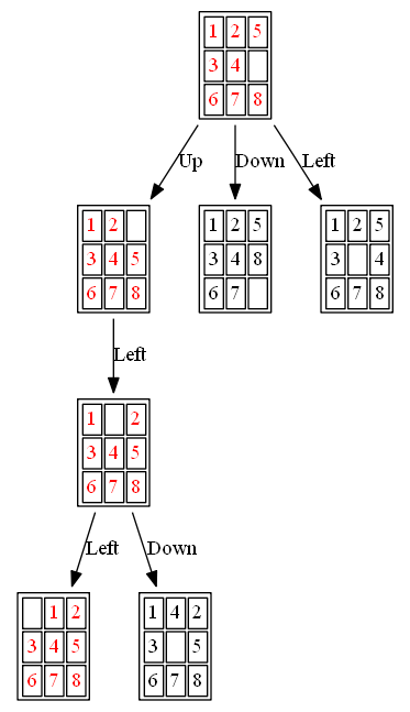
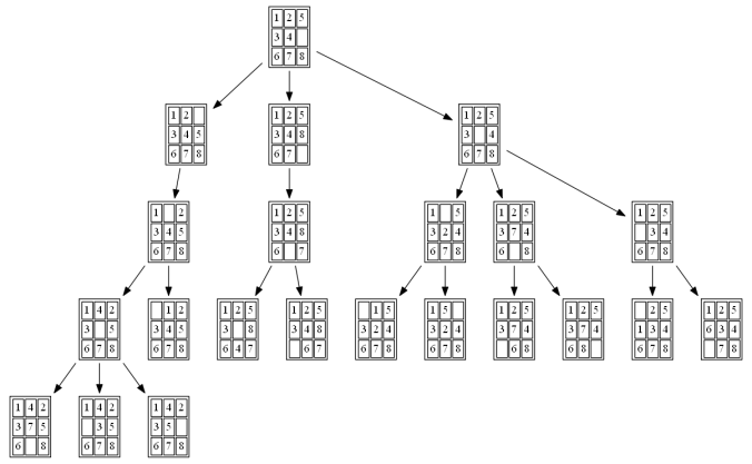
Example 1: Initial State: 1,2,5,3,4,0,6,7,8
(1) BFS

The path to the goal node with BFS is shown in the following figure:
The nodes expanded by BFS (also the nodes that are in the fringe / frontier of the queue) are shown in the following figure:
(2) DFS
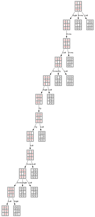
The path to the goal node with DFS is shown in the following figure:

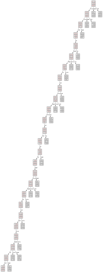
(3) A*

The path to the goal node with A* (also the nodes expanded by A*) is shown in the following figure:

(4) ID-A*

The path to the goal node (as well as the nodes expanded) with ID-A* is shown in the following figure:

Now let’s try a little more complex examples:
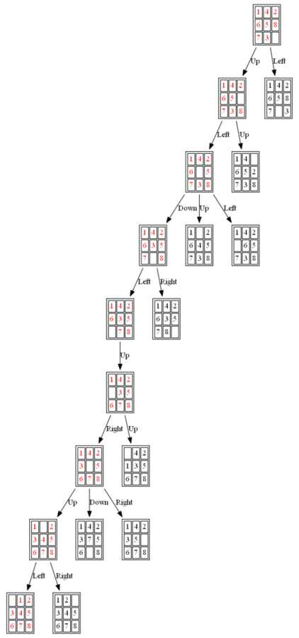
Example 2: Initial State: 1,4,2,6,5,8,7,3,0
(1) A*

The path to the goal node with A* is shown in the following figure:
All the nodes expanded by A* (also the nodes that are in the fringe / frontier of the queue) are shown in the following figure:
(2) BFS
The path to the goal node with BFS is shown in the following figure:

All the nodes expanded by BFS are shown in the following figure:
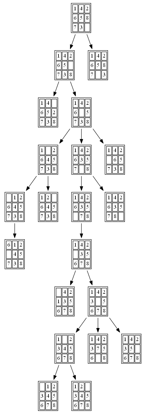
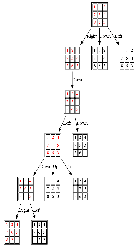
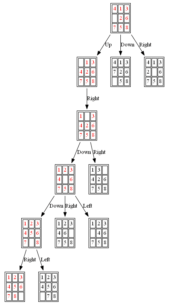
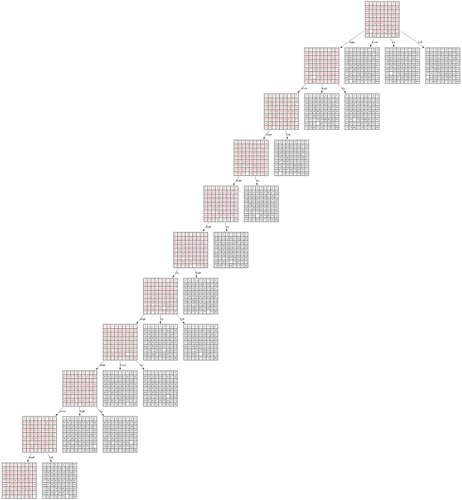
Example 3: Initial State: 1,0,2,7,5,4,8,6,3
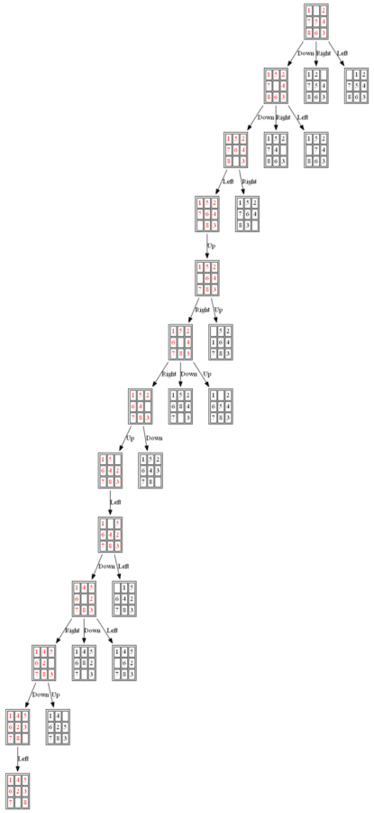
(1) A*
The path to the goal node with A* is shown in the following figures:
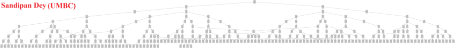
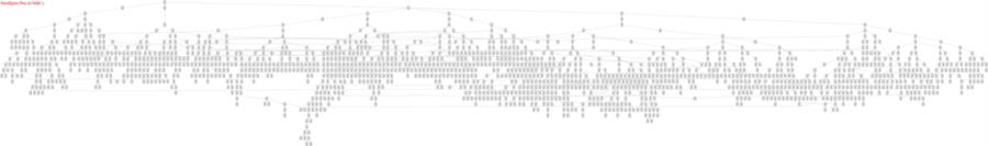
The nodes expanded by A* (also the nodes that are in the fringe / frontier of the priority queue) are shown in the following figure (the tree is huge, use zoom to view it properly):

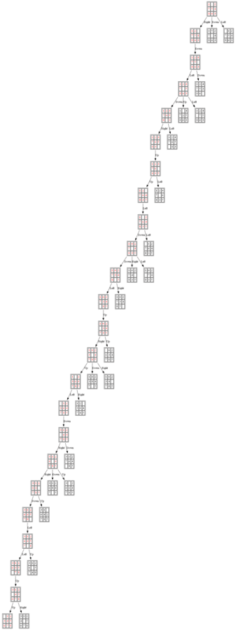
(2) ID-A*

The nodes expanded by ID-A* are shown in the following figure (again the tree is huge, use zoom to view it properly):
The same problem (with a little variation) also appeared a programming exercise in the Coursera Course Algorithm-I (By Prof. ROBERT SEDGEWICK, Princeton). The description of the problem taken from the assignment is shown below (notice that the goal state is different in this version of the same problem):
Write a program to solve the 8-puzzle problem (and its natural generalizations) using the A* search algorithm.
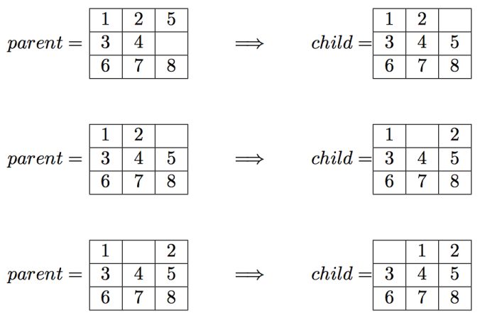
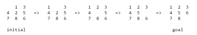
The problem. The 8-puzzle problem is a puzzle invented and popularized by Noyes Palmer Chapman in the 1870s. It is played on a 3-by-3 grid with 8 square blocks labeled 1 through 8 and a blank square. Your goal is to rearrange the blocks so that they are in order. You are permitted to slide blocks horizontally or vertically into the blank square. The following shows a sequence of legal moves from an initial board position (left) to the goal position (right).
Best-first search. We now describe an algorithmic solution to the problem that illustrates a general artificial intelligence methodology known as the A* search algorithm. We define a state of the game to be the board position, the number of moves made to reach the board position, and the previous state. First, insert the initial state (the initial board, 0 moves, and a null previous state) into a priority queue. Then, delete from the priority queue the state with the minimum priority, and insert onto the priority queue all neighboring states (those that can be reached in one move). Repeat this procedure until the state dequeued is the goal state. The success of this approach hinges on the choice of priority function for a state. We consider two priority functions:
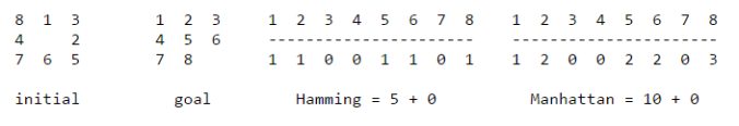
- Hamming priority function. The number of blocks in the wrong position, plus the number of moves made so far to get to the state. Intutively, a state with a small number of blocks in the wrong position is close to the goal state, and we prefer a state that have been reached using a small number of moves.
- Manhattan priority function. The sum of the distances (sum of the vertical and horizontal distance) from the blocks to their goal positions, plus the number of moves made so far to get to the state.
For example, the Hamming and Manhattan priorities of the initial state below are 5 and 10, respectively.
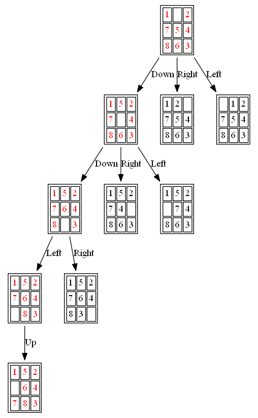
(1) The following 8-puzzle is solvable with A* / Manhattan heuristic in 5 steps, as shown below:
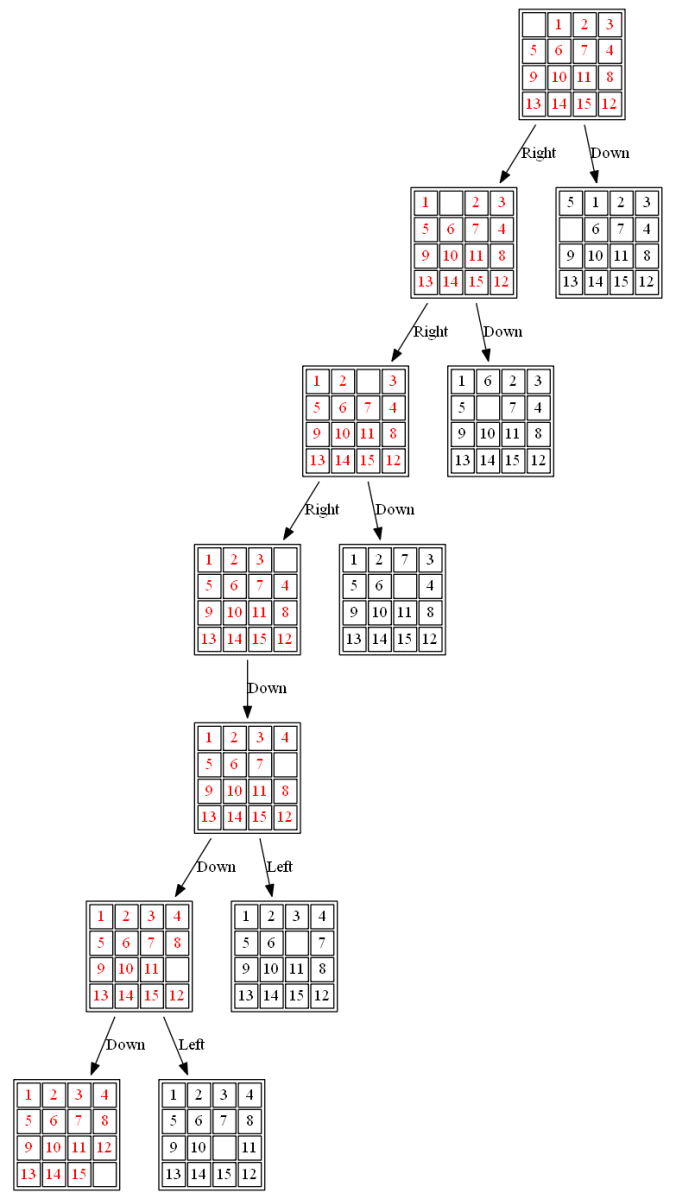
(2) The following 15-puzzle is solvable in 6 steps, as shown below:
(3) The following 80-puzzle is solvable in 10 steps, as shown below:
%20in%20Python)