
TLDR: Neural Networks are powerful but complex and opaque tools. Using Topological Data Analysis, we can describe the functioning and learning of a convolutional neural network in a compact and understandable way. The implications of the finding are profound and can accelerate the development of a wide range of applications from self-driving everything to GDPR.
Introduction
Neural networks have demonstrated a great deal of success in the study of various kinds of data, including images, text, time series, and many others. One issue that restricts their applicability, however, is the fact that it is not understood in any kind of detail how they work. A related problem is that there is often a certain kind of overfitting to particular data sets, which results in the possibility of adversarial behavior. For these reasons, it is very desirable to develop methods for developing some understanding of the internal states of the neural networks. Because of the very large number of nodes (or neurons) in the networks, this becomes a problem in data analysis, specifically for unsupervised data analysis.
In this post, we will discuss how topological data analysis can be used to obtain insight into the working of convolutional neural networks (CNN’s). Our examples are exclusively from networks trained on image data sets, but we are confident that topological modeling can just as easily explain the workings of many other convolutional nets. This post describes joint work between Rickard Gabrielsson and myself.
First, a couple of words about neural networks. A neural network is specified by a collection of nodes and directed edges. Some of the nodes are specified as input nodes, others as output nodes, and the rest as internal nodes. The input nodes are the features in a data set. For example, in the case of images, the input nodes would be the pixels in a particular image format. In the case of text analysis, they might be individual words.
Suppose that we are given a data set and a classification problem for it, such as the MNIST data set of images of hand drawn digits, where one is attempting to classify each image as one of the digits 0 through 9. Each node of the network corresponds to a variable which will take different values (called activations) depending on values assigned to the input nodes. So, each data point produces values for every internal and output node in the neural network. The values at each node of the network are determined by a system of numerical weights assigned to each of the edges. The value at a node (in Figure 1, node Z) is determined by a function of the nodes which connect to it by an edge (in Figure 1, nodes A,B,C,D).
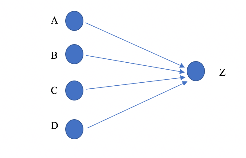
Figure 1. An example of nodes in a network
The activation at the rightmost node (Figure 1, node Z) is computed as a function of the activations of the four nodes A,B,C, and D, based on the weights assigned to the four edges. One possible such function would be
(wAxA+wBxB+ wCxC+wDxD)
where wA, wB, wC, and wD are the weights associated to the edges AZ, BZ, CZ, and DZ, xA, xB, xC,and xD, are the activations at the nodes A,B,C, and D, respectively, and is a fixed function, which typically has its range between 0 and 1, and is typically monotonic. A choice of the weights determines a complex formula for each of the nodes (including the output nodes) in terms of the values at the input nodes. Given a particular output function of the inputs, an optimization procedure is then used to select all the weights in such a way as to best fit the given output function. To each node in the right hand layer one then associates its weight matrix, i.e. the matrix of the weights of all the incoming edges.
Understanding Weights of a Trained Network
There is a particular class of neural networks that are well adapted to databases of images, called convolutional neural networks. In this case, the input nodes are arranged in a square grid corresponding to the pixel array for the format of the images that comprise the data. The nodes are composed in a collection of layers, so that all edges whose initial node is in the i-th layer have their terminal node in the (i+1)-st layer. A layer is called convolutional if it is made up of a collection of square grids identical to the input layer, and it is understood that the weights at the nodes in each such square grid (a) involve only nodes in the previous layer that are very near to the corresponding node and (b) obey a certain homogeneity condition, so that for each square grid in layer i, the weights attached to a given node are identical to those for another node in the same grid, but translated to its surrounding neurons. Sometimes intermediate layers called pooling layers are introduced between convolutional layers, and in this case the higher convolutional layers are smaller square grids. Here is a schematic picture that summarizes the situation.
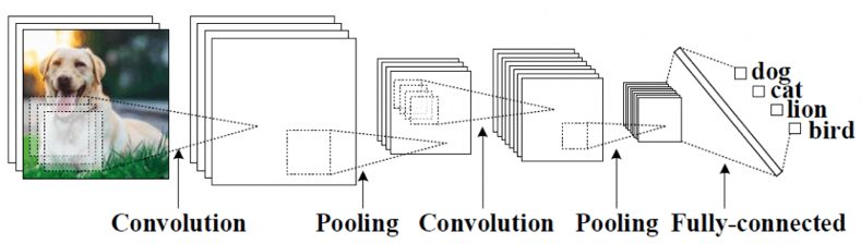
Figure 2: The structure of a Convolutional Neural Network
In order to discern the underlying behavior of a CNN we need to understand the weight matrices. Consider the dataset where each datapoint is the weight matrix associated with a neuron in the hidden layer. We collect data from all the grids in a fixed layer, and do this over many different trainings of the same network on the same training data. Finally, we perform topological data analysis on the set of weight matrices.
By performing TDA on the weight matrices we can, for the first time, understand the behavior of the CNN, proving, independently, that the CNN faithfully represents the underlying distributions occurring in natural images.
Here is how it is done.
To start with we need to find useful structure from a topological perspective. To achieve that, we consider only the points of sufficiently high density (computed using simple proxy for Gaussian density as in the 2008 paper, called codensity). We begin by looking at, the 1st convolutional layer in a two-layer convolutional neural network. It produces the topological model shown in Figure 3.
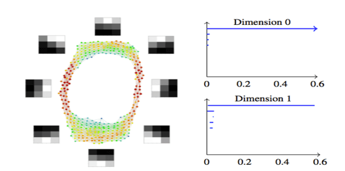
Figure 3 – TDA Mapper model colored by density of the filters. Shows a) the edges organize in a circle (i.e. there are filters for each direction) and b) the model over-represents the horizontal and vertical edges.
Note that the model is circular.
The barcodes shown on the right are persistent homology barcodes, which are topological shape signatures that show that the data set in fact has this shape, and that it is not an artifact of the model constructed using Mapper. The explanation for the shape is also shown in the image by labeling parts of the model with the mean of the corresponding set of weight matrices. What is very interesting about this model is that it is entirely consistent with what is found in a study of the statistics of 3×3 patches in grayscale natural images, as well as what is found in the so-called primary visual cortex, a component of the visual pathway that connects directly with the retina1.
Put more simply, the topological model describes the CNN in such a way that we can independently confirm that it matches how humans see the world, and matches with density analysis of natural images.
This analysis in Figure 3 was performed on the MNIST data set. A related analysis, performed on the CIFAR 10 data set, gives the following diagram and persistence barcode.
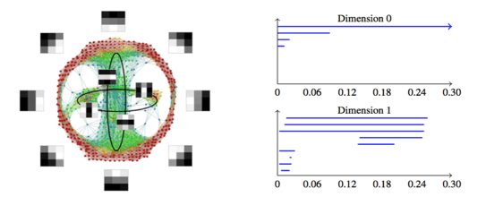
Figure 4: Note that the additional complexity of the CIFAR 10 data set is shown in the horizontal and vertical lines and captures more detail than edges alone.
This comes from the first convolutional layer. Neurons that are tuned to these line patches also exist in the mammalian primary visual cortex. This provides a quantitative perspective of the qualitative aspects that we have come to associate with vision. There are, however, opportunities to go deeper.
Understanding Weights as They Change During Training
Now that we have proven, using TDA, that CNN’s can mimic the distribution of data sets occurring in natural images, we can turn our attention to the study of what happens over the course of the learning process. Figure 5 below is obtained by computing topological models in the first and second layer of a convolutional neural network on the CIFAR 10 data set used above, and then displaying models for both the first and second layers at various numbers of learning iterations.
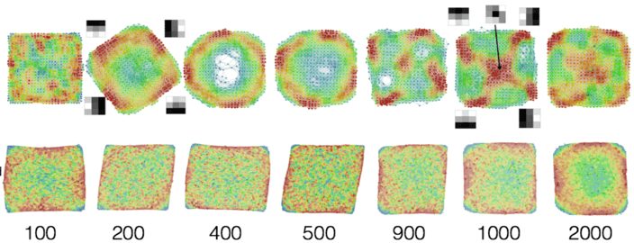
Figure 5: Topological models at various stages of neural net learning
We use the coloring of the model to obtain information about what is happening. The coloring reflects the number of data points in a node, so we can consider the red portion as the actual model, where the rest contains weight matrices that appear less often.
The top row reflects the first layer, and one observes that it quickly discovers the circular model mentioned above, after 400 and 500 iterations of the optimization algorithm. What then starts to happen, though, is that the circle devolves instead into a more complex picture, which includes the patches corresponding to horizontal and vertical patches, but now also including a more complex pattern in the center of the model after 1,000 iterations. In the second layer, on the other hand, we see that during the first rounds of the iterations, there is only a weak pattern, but that after 2,000 iterations there appears to be a well- defined circular model. Our hypothesis is that the second layer has “taken over” from the first layer, which has moved to capture more complex patches. This is an area for future potential research.
This demonstrates the capability of using topological data analysis to monitor and provide insight into the learning process of a neural network – something that has been highly elusive until now.
Higher Level Weight Matrices
This method also works on deeper networks (i.e. networks including more layers). Deeper networks are organized in a way that resembles the organization of the visual pathway in humans or primates. It is understood that the pathway has a number of components, including the retina, the so-called primary visual cortex or V1, and various higher components. It is thought that the primary visual cortex acts as an edge and line detector, and that the higher components detect more complex shapes, perhaps seen at larger scales. The picture below is the result of a study of the layers in an already trained network, VGG 16, that has been trained on the ImageNet data set referenced by J. Deng, W. Dong, R. Socher, L.-J. Li, K. Li, and L. FeiFei. Here we display the 2nd through the 13th convolutional layers, given as topological models.
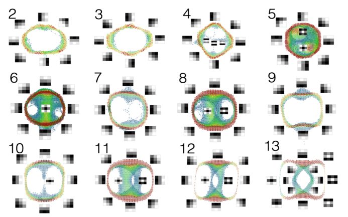
Figure 6: A 13 layer neural network represented by topological data analysis
Notice that the 2nd and 3rd layers are clearly very similar to the circular models found in the model trained on the MNIST data set. At the fourth layer, we have a circular model, but that also includes some lines in the middle of a background. These reflect the “secondary circles” found in the 2008 paper. At the higher levels, though, very interesting patterns are developed that include line crossings and “bulls eyes”, which are not seen in the analysis in the 2008 paper, nor in the primary visual cortex.
What these topological models tell us is that the convolutional neural network is not only mimicking the distribution of real world data sets, but is also able to mimic the development of the mammalian visual cortex.
While CNN’s are notoriously difficult to understand, topological data analysis provides a way to understand, at a macro scale, how computations within a neural network are being performed. While this work is applied to image data sets, the use of topological data analysis to explain the computations of other neural networks also applies.
By providing a compression of a large set of states into a much smaller and more comprehensible model, topological data analysis, can be used to understand the behavior and function of a broad range neural networks.
On a practical basis, this approach may facilitate our understanding of the behavior of (and subsequent debugging of) any number of vision problems from drone flight to self-driving automobiles to matters relating to GDPR. The details of this study will appear in due course.
References
- D. Hubel, Eye, Brain and Vision, Scientific American library series, No. 22, Scientific American Library/Scientific American Books, 1995