
In an earlier blog, “Need for DYNAMICAL Machine Learning: Bayesian exact recursive estimation”, I introduced the need for Dynamical ML as we now enter the “Walk” stage of “Crawl-Walk-Run” evolution of machine learning. First, I defined Static ML as follows: Given a set of inputs and outputs, find a static map between the two during supervised “Training” and use this static map for business purposes during “Operation”. I made the following points using IoT as an example.
Static ML:
- What is normal for a machine (or the System under observation) is environment-dependent and ever-changing in real life!
- · Systems “wander” about in a normal zone . . . However, such safe-range determination is ad-hoc since we do not have the actual experience of this particular machine and its own range of “normal” behavior as it ages. Consequence of the system’s evolution within its normal range for Static ML then is the possibility of increased False Positive events!
- With the Static ML solution, when “abnormal” is indicated, prediction of what the machine’s condition (via ML “map” output) will not be possible since the System has changed (as the detection of Abnormal indicated).
- · In summary, Static ML is adequate for one-off detection (and subsequent offline intervention) IF your business has a high tolerance for false positives.
Dynamical ML solution involves State-Space data model (more below). What more does a Dynamical ML solution offer?
- · States are a sort of “meta”-level description of the machine under monitoring in an IoT application. States are less variable than external measurements; this is an indication that States are capturing something “deeper” about the underlying system.
- Consider any misclassification event (detected as measurements exceeding thresholds). If you observe the State trajectories at the same instant of misclassification and find that there are hardly any changes in the States, this indicates that this event is most likely a False Positive (you do not have to send a technician to troubleshoot the machine)!
- With growing experience, changes in States can be connected to the nature of change in the machine – both when normal and abnormal, providing a level of remote troubleshooting minimizing “truck rolls”.
- · New normal: Let us say that the machine usually process aluminum but switched to titanium work pieces (vibration and temperature signals will be very different). Dynamical ML will adapt to the new normal instead of having to retrain the static ML map. With Static ML, the option would have been (1) to train Static ML for multiple types of work pieces separately and switch the map when work piece is switched – a tedious and error-prone solution or (2) to train the Static ML map for all potential work piece types – which will “smear out” the map and make it less accurate overall; in probabilistic terms, this is caused by non-homogeneity of data.
If you contribute to the view that true learning is “generalization from past experience AND the results of new action” and therefore ML business solutions ought to be like flu shots (adjust the mix based on response effect and apply on a regular basis), then every ML application is a case of Dynamical Machine Learning.
How DYNAMICAL Machine Learning is practiced is discussed in Generalized Dynamical Machine Learning and associated articles describing the theory, algorithms, examples and MATLAB code (in Systems Analytics: Adaptive Machine Learning workbook).
Now that we have the basics in hand, let us turn to the distinction between Static and Dynamical ML. Since the publication of my “Need for Dynamical ML” blog, I have had various readers ask, “What is the REAL difference between the two?”. The main confusion seems to be due to the fact that learning rules in most Static ML algorithms are step-by-step or iterative – is this not a case of “dynamic” learning? Fair question . . . there IS some over-lap here and hence the confusion!
The main distinction to keep in mind are between (1) Data Models and (2) Learning Methods. They are disjoint aspects but have commonalities – hence the tendency to conflate the two and the resulting lack of clarity. Let me explain . . .
From first principles . . .
Machine Learning is a procedure to find the map, “f”.

Given N pairs of {x, y}, where as usual, ‘x‘ are the input features and ‘y’ is the desired output in the Training Set, our problem is to find ‘f’ where ‘f’ is a linear or nonlinear and time-invariant or time-varying function.
yi = f(xi) + ei where i = 1, 2, . . ., N. Here, ei is an additive white noise with zero mean and variance = se2.
A complete solution from Bayesian estimation perspective of the unknown function, f, is the Conditional Expectation (mean) of y given regressor, x.
The above is a complete statement of the problem and solution of Machine Learning.
Map, “f”, that we find can be in two forms: (1) Parametric where “f” can be explicitly written out (such as a multiple linear regression equation) or (2) Non-parametric where “f” is not explicitly defined (such as multi-layer perceptron, deep neural network, etc.). Consider the parametric, time-invariant/ varying case of ML below.
Parametric model of the map, “f”, is often called “Data Model”. Data Model contains parameters (or model coefficients) that are either time-invariant or time-varying. ML is the exercise of finding the Parameters of a chosen Data Model from known data. Once “learned”, this model or map is used with new data for useful tasks such as classification and regression during “operation”.
In Machine Learning, (1) a Data Model is chosen; (2) a Learning Method is selected to obtain model parameters & (3) data are processed in a “batch” or “in-stream” (or sequential) mode.
(1) Data Model: There are 3 classes of Data Models: Static, Dynamical and Time-Varying Dynamical.
Static Model: Regression models used in ML are usually static, defined as follows.
Multiple Linear Regression Model: y = a0 + a1 x1 + a2 x2 + . . . + aM xM + w
We know that it is static because there are NO time variables in the equation. Let us make the lack of time dependence explicit.
y[n] = a0 + a1 x1[n] + a2 x2[n] + . . . + aM xM[n] + w[n]
It is the same time index, n, on both sides of the equation and hence there is no dependence on time which we call a “Static” model.
Dynamical Model: Box & Jenkins time series model is a familiar dynamical model.
y[n] = – a1 y[n-1] – . . . – aD y[n-D] + b1 x1[n] + . . + bM xM[n-M+1] + e[n]
This is the classic ARMA model. There are delayed time indices on the right-hand side (but note that the coefficients, a & b, are constants). This provides “memory” to the model and hence the output, y, is variable over time. Therefore, they are called Dynamical models.
Time-Varying Dynamical Model: In the model above, if the coefficients, a & b, were not constant but indexed by time, n, that is an example of a time-varying dynamical model. We choose to use a more flexible model called State Space model.
State-space Model:
s[n] = A s[n-1] + D q[n-1]
y[n] = H[n] s[n] + r[n]
Difference between Dynamical & Time-Varying Dynamical models:
The same sequence of inputs applied to a Dynamical model at time=T1 and time=T2 will produce the SAME output at T1 and T2. Whereas, in the case of a time-varying Dynamical model, output at T1 and T2 will be different!
Detailed discussion of such models is available in the book, “SYSTEMS Analytics”, but we will note here that output, y, is a function of ‘s’ (so-called “States”) and the first equation shows that these States evolve according to a Markov process. This is akin to allowing the equation coefficients in the ARMA model to evolve over time, thus accommodating time-variability of the dynamics of the data.
[The only other possibility that these Data Models do not accommodate is non-linearity. By choice, we will not consider the nonlinear case here.]
(2) Learning Methods: There are 3 classes of Learning Methods: Block, Recursive & Real-time Recursive.
KEY section: Most of the confusion between Static and Dynamical ML arise in the context of Learning!
Block methods are well known. Pseudo-inverse is one way to solve for constant coefficients of a multiple linear regression Static model.
Recursive method is best understood by recalling Programming 101 course example; x! = (x-1)! * x with 0!=1. The formula “calls itself” to get the answer for any ‘x’. Method of steepest descent is an UN-constrained optimization method that is used to obtain the weights of a multilayer perceptron, for example. SYSTEMS Analytics book under Formal Learning Methods section (page 51) explains more details – Jacobian and Hessian matrices come into play in advanced Gradient Search methods.
In Gradient Descent methods, same data are presented multiple times till some local or global optimum is reached. Now comes the subtle distinction that creates the confusion – there is another CLASS of recursive learning methods where the data is presented ONLY ONCE.
To create a clear distinction, we will call the recursive learning methods when data is processed only once as “Real-time Recursive” Learning methods. Here are some well-known examples.
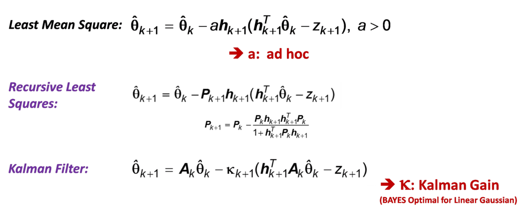
As you can see, they all have the recursive form. What is different is the 2nd term on the RHS, the “correction” term. They can be ad hoc, approximate or exact; exact in the sense that after N data points are processed, Block and Recursive methods provide identical answers!
Coming to the Kalman Filter case above, it is well known that it is the Bayesian optimal solution for linear Gaussian case. Once the conditional posterior distribution of ‘y’ in the State-space data model is estimated, we still need its “point” estimate for practical applications (“what is the class label?”). Such scalar-valued result is obtained from Statistical Decision Theory by minimizing a loss function that incorporates the posterior distribution (as an example, for a quadratic loss function, the optimum is the expected value which will result in Minimum Mean Squared Error). This is how this “constrained” minimization/ optimization problem is connected to the UN-constrained optimization of Steepest Descent method.
In recursive Bayesian solution, we treat the posterior distribution of the previous time step as the prior for the current time step. Both Bayesian block and recursive methods will produce identical results after processing the exact same amount of data. However, Recursive Bayesian method has some additional useful properties (Sarkka, 2013).
- On-line learning solution. Updated using new pieces of information as they arrive.
- Because each step in the recursive estimation is a full Bayesian update step, block Bayesian inference is a special case of the general recursive Bayesian inference.
–> “Real-time Recursive Learning”
- Due to the sequential nature of estimation, we can model the effect of time on the parameters of the State-space data model.
For a complete discussion of Kalman Filter use for Dynamical machine learning, see SYSTEMS Analytics book.
(3) Processing Modes: There are 2 classes: Batch and In-Stream modes.
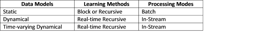
Batch mode processing utilizes Block or Recursive Learning methods for Static Data models.
However, Dynamical and Time-Varying Dynamical Data models REQUIRE the use of “Real-time Recursive” Learning in a Sequential or In-Stream processing mode.
Batch mode processing is well known in all Machine Learning techniques for supervised learning of neural networks, SVM, etc. A full exposition of Real-time Recursive algorithms of various kinds (including nonlinear) is available in Generalized Dynamical Machine Learning. Here is an example of one of my favorite algorithms that I affectionately refer to as “Rocket” Kalman (Recurrent Kernel-projection Time-varying Kalman method)!
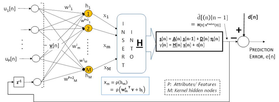
In this configuration for pattern classification, attributes/ features, u[n], that may have temporal dependence are processed (once) in real-time as each u[n] arrives. The Real-time Recursive algorithm (Kalman with modifications for the time-varying dynamical case) processes the current data (and “memorized” past inputs and outputs) and provides a “class label” prediction sequentially.
Machine Learning frameworks are summarized in this table.
 Dynamical Machine Learning requires “real-time recursive” learning algorithms and time-varying data models. A class of solutions for Dynamical ML has been developed recently and is available in Generalized Dynamical Machine Learning.
PG Madhavan, Ph.D. – “Data Science Player+Coach with deep & balanced track record in Machine Learning algorithms, products & business”