
This article was written by Prashant Gupta.
One of the major aspects of training your machine learning model is avoiding overfitting. The model will have a low accuracy if it is overfitting. This happens because your model is trying too hard to capture the noise in your training dataset. By noise we mean the data points that don’t really represent the true properties of your data, but random chance. Learning such data points, makes your model more flexible, at the risk of overfitting.
The concept of balancing bias and variance, is helpful in understanding the phenomenon of overfitting.
One of the ways of avoiding overfitting is using cross validation, that helps in estimating the error over test set, and in deciding what parameters work best for your model.
This article will focus on a technique that helps in avoiding overfitting and also increasing model interpretability.
Regularization
This is a form of regression, that constrains/ regularizes or shrinks the coefficient estimates towards zero. In other words, this technique discourages learning a more complex or flexible model, so as to avoid the risk of overfitting.
A simple relation for linear regression looks like this. Here Y represents the learned relation and β represents the coefficient estimates for different variables or predictors(X).
Y ≈ β0 + β1X1 + β2X2 + …+ βpXp
The fitting procedure involves a loss function, known as residual sum of squares or RSS. The coefficients are chosen, such that they minimize this loss function.
Now, this will adjust the coefficients based on your training data. If there is noise in the training data, then the estimated coefficients won’t generalize well to the future data. This is where regularization comes in and shrinks or regularizes these learned estimates towards zero.
Ridge Regression
Now, the coefficients are estimated by minimizing this function. Here, λ is the tuning parameter that decides how much we want to penalize the flexibility of our model. The increase in flexibility of a model is represented by increase in its coefficients, and if we want to minimize the above function, then these coefficients need to be small. This is how the Ridge regression technique prevents coefficients from rising too high. Also, notice that we shrink the estimated association of each variable with the response, except the intercept β0, This intercept is a measure of the mean value of the response when xi1 = xi2 = …= xip = 0.
When λ = 0, the penalty term has no effect, and the estimates produced by ridge regression will be equal to least squares. However, as λ→∞, the impact of the shrinkage penalty grows, and the ridge regression coefficient estimates will approach zero. As can be seen, selecting a good value of λ is critical. Cross validation comes in handy for this purpose. The coefficient estimates produced by this method are also known as the L2 norm.
The coefficients that are produced by the standard least squares method are scale equivariant, i.e. if we multiply each input by c then the corresponding coefficients are scaled by a factor of 1/c. Therefore, regardless of how the predictor is scaled, the multiplication of predictor and coefficient(Xjβj) remains the same. However, this is not the case with ridge regression, and therefore, we need to standardize the predictors or bring the predictors to the same scale before performing ridge regression.
Lasso
Lasso is another variation, in which the above function is minimized. Its clear that this variation differs from ridge regression only in penalizing the high coefficients. It uses |βj|(modulus)instead of squares of β, as its penalty. In statistics, this is known as the L1 norm.
Lets take a look at above methods with a different perspective. The ridge regression can be thought of as solving an equation, where summation of squares of coefficients is less than or equal to s. And the Lasso can be thought of as an equation where summation of modulus of coefficients is less than or equal to s. Here, s is a constant that exists for each value of shrinkage factor λ. These equations are also referred to as constraint functions.
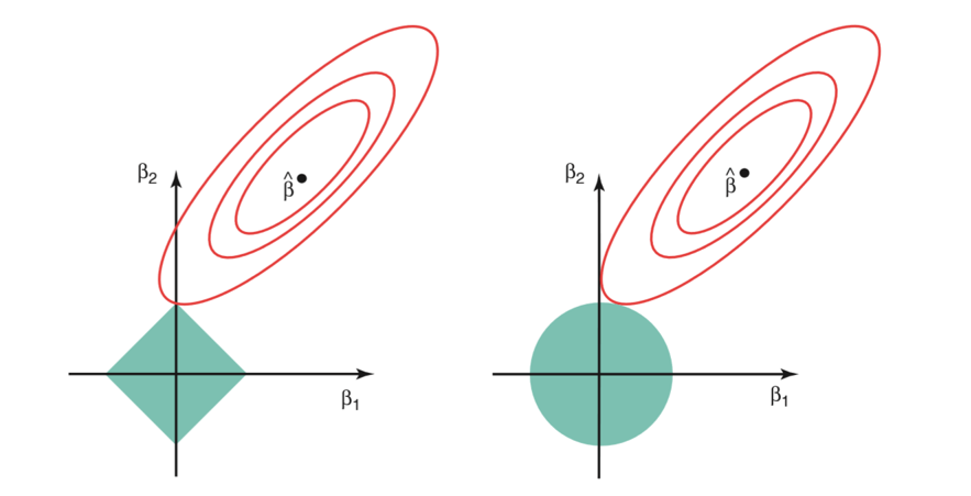
Consider their are 2 parameters in a given problem. Then according to above formulation, the ridge regression is expressed by β1² + β2² ≤ s. This implies that ridge regression coefficients have the smallest RSS(loss function) for all points that lie within the circle given by β1² + β2² ≤ s.
Similarly, for lasso, the equation becomes,|β1|+|β2|≤ s. This implies that lasso coefficients have the smallest RSS(loss function) for all points that lie within the diamond given by |β1|+|β2|≤ s.
To read the whole article, with illustrations, click here. For another article on the same topic, follow this link.