Regression, Logistic Regression and Maximum Entropy

One of the most important tasks in Machine Learning are the Classification tasks (a.k.a. supervised machine learning). Classification is used to make an accurate prediction of the class of entries in the test set (a dataset of which the entries have not been labelled yet) with the model which was constructed from a training set. You could think of classifying crime in the field of Pre-Policing, classifying patients in the Health sector, classifying houses in the Real-Estate sector. Another field in which classification is big, is Natural Lanuage Processing (NLP). This is the field of science with the goal to makes machines (computers) understand (written) human language. You could think of Text Categorization, Sentiment Analysis, Spam detection and Topic Categorization.

For classification tasks there are three widely used algorithms; the Naive Bayes, Logistic Regression / Maximum Entropy and Support Vector Machines. We have already seen how the Naive Bayes works in the context of Sentiment Analysis. Although it is more accurate than a bag-of-words model, it has the assumption of conditional independence of its features. This is a simplification which makes the NB classifier easy to implement, but it is also unrealistic in most cases and leads to a lower accuracy. A direct improvement on the N.B. classifier, is an algorithm which does not assume conditional independence but tries to estimate the weight vectors (feature values) directly.

This algorithm is called Maximum Entropy in the field of NLP and Logistic Regression in the field of Statistics.

Maximum Entropy might sounds like a difficult concept, but actually it is not. It is a simple idea, which can be implemented with a few lines of code. But to fully understand it, we must first go into the basics of Regression and Logistic Regression.

1. Regression Analysis

Regression Analysis is the field of mathematics where the goal is to find a function which best correlates with a dataset. Lets say we have a dataset containing $n$ datapoints; $X = ( x^{(1)}, x^{(2)}, .., x^{(n)} )$ . For each of these (input) datapoints there is a corresponding (output) $y^{(i)}$ -value. Here the $x$ -datapoints are called the independent variables and $y$ the dependent variable; the value of $y^{(i)}$ depends on the value of $x^{(i)}$ , while the value of $x^{(i)}$ may be freely chosen without any restriction imposed on it by any other variable.
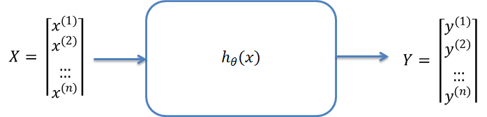
The goal of Regression analysis is to find a function $f(X)$ which can best describe the correlation between $X$ and $Y$ . In the field of Machine Learning, this function is called the hypothesis function and is denoted as $h_{\theta}(x)$ .

If we can find such a function, we can say we have successfully build a Regression model. If the input-data lives in a 2D-space, this boils down to finding a curve which fits through the datapoints. In the 3D case we have to find a plane and in higher dimensions a hyperplane.

To give an example, lets say that we are trying to find a predictive model for the success of students in a course called Machine Learning. We have a dataset $Y$ which contains the final grade of $n$ students. Dataset $X$ contains the values of the independent variables. Our initial assumption is that the final grade only depends on the studying time. The variable $x^{(i)}$ therefore indicates how many hours student $i$ has studied. The first thing we would do is visualize this data:

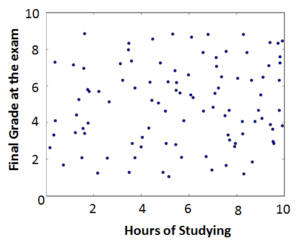
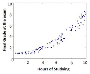
If the results looks like the figure on the left, then we are out of luck. It looks like the points are distributed randomly and there is not correlation between $Y$ and $X$ at all. However, if it looks like the figure on the right, there is probably a strong correlation and we can start looking for the function which describes this correlation.

This function could for example be:

$h_{\theta}(X) = \theta_0+ \theta_1 \cdot x$

$h_{\theta}(X) = \theta_0 + \theta_1 \cdot x^2$

where $\theta$ are the dependent parameters of our model.

1.1. Multivariate Regression

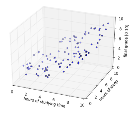
Evaluating the results from the previous section, we may find the results unsatisfying; the function does not correlate with the datapoints strong enough. Our initial assumption is probably not complete. Taking only the studying time into account is not enough. The final grade does not only depend on the studying time, but also on how much the students have slept the night before the exam. Now the dataset contains an additional variable which represents the sleeping time. Our dataset is then given by $X = ( (x_1^{(1)}, x_2^{(1)}), (x_1^{(2)}, x_2^{(2)}), .., (x_1^{(n)}, x_2^{(n)}) )$ . In this dataset $x_1^{(i)}$ indicates how many hours student $i$ has studied and $x_2^{(i)}$ indicates how many hours he has slept.

See the rest of the blog here, including Linear vs Non-linear, Gradient Descent, Logistic Regression, and Text Classification and Sentiment Analysis.